bamm

The bamm package is an R package designed to create and operate on large (tens of millions of cells) matrices regarding to each element of the $\textbf{BAM}$ scheme, for example, the adjacency matrix (connectivity matrix), and the niche suitability matrices.

The following vignette presents the basic functions and methods of the bamm package. The package has three main functionalities related to each element of the BAM scheme.

library(bamm)

A functions

Convert niche models to sparse matrices

The package uses sparse matrices to represent those objects which allows it to optimize computers memory and make important speed ups in computation times by eliminating operations on zero elements. The basic function of the package is model2sparse which converts a raster model to an setA class

model_path <- system.file("extdata/Lepus_californicus_cont.tif",
                          package = "bamm")
model <- raster::raster(model_path) 
# binary model
model_bin <- model > 0.7
sparse_mod <- bamm::model2sparse(model = model_bin)

The slots of the object are

sparse_mod
#> Set A of the BAM digram it contains 8 slots 
#> 
#> @niche_model: a niche model:
#> 
#> class      : RasterLayer 
#> dimensions : 91, 159, 14469  (nrow, ncol, ncell)
#> resolution : 0.2, 0.2  (x, y)
#> extent     : -118.4042, -86.60417, 14.51846, 32.71846  (xmin, xmax, ymin, ymax)
#> crs        : +proj=longlat +datum=WGS84 +no_defs 
#> source     : memory
#> names      : layer 
#> values     : 0, 1  (min, max)
#> 
#> @suit_threshold: Threshold value used to binarize model@cellIDs: ids of the cells that have values (4281 pixels) 
#> 
#> @suit_values: Suitability values of the continuous model
#> 
#> @sparse_model: A sparse square matrix of  4281 x 4281 entries 
#> 
#> @coordinates: Pixel centroid coordinates of the model

M functions

Connectivity matrix

The function to estimate connectivity between pixels of a given raster is adj_mat, (generally is the M area but can be any matrix); it uses sparse adjacency matrices.

 # Adjacency matrix from a niche model


adj_mod <- adj_mat(sparse_mod,ngbs=1,eigen_sys = T)
adj_mod
#> Set M of the BAM digram it contains 7 slots 
#> 
#> @coordinates: A matrix with longitude and latitude values of each cell of the raster area
#> 
#>              x        y
#> [1,] -115.9042 32.61846
#> [2,] -115.7042 32.61846
#> [3,] -115.5042 32.61846
#> [4,] -115.3042 32.61846
#> [5,] -115.1042 32.61846
#> [6,] -114.9042 32.61846
#> @eigen_val: Eigen values of the connectivity matrix M
#> 
#> [1] 7.975459
#> @eigen_vec: Eigen vector of the connectivity matrix M
#> 
#>               [,1]
#> [1,] -8.640620e-11
#> [2,] -1.555028e-10
#> [3,] -2.564191e-10
#> [4,] -4.169028e-10
#> [5,] -6.556495e-10
#> [6,] -8.733471e-10

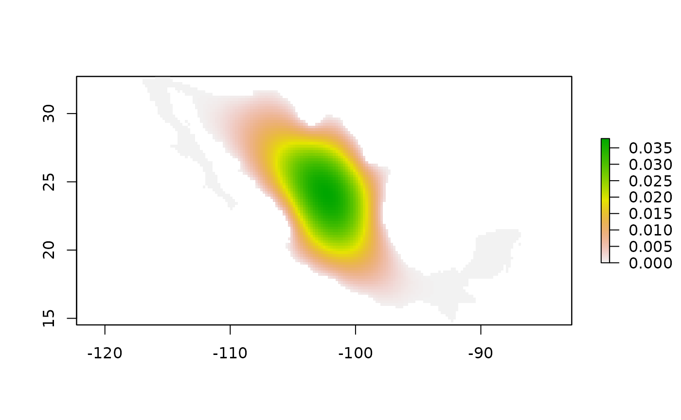
The map of the connectivity matrix adj_mod is

model_eig <- model
model_eig[sparse_mod@cellIDs] <- abs(adj_mod@eigen_vec)
raster::plot(model_eig)

Fig. 1 Connectivity map of adj_mod object. Here green color means more connected.

AM objects

These are objects that combine SetA and SetM .

Connectivity Suitability diagram

Estimates the connectivity suitability and dispersal diagram. It shows the number of geographic clusters as a function of dispersal and suitability.

clustersin <- bamm::bam_clusters(model=sparse_mod,
                                ngbs=1,plot_model=FALSE)

The function returns the following slots

clustersin
#> Object of class csd it contains 3 slots: 
#> 
#> @connections: Geographic clusters data.frame 
#> 
#>           x        y clusterID cluster_size
#> 1 -116.3042 32.41846         1           37
#> 2 -116.7042 32.21846         1           37
#> 3 -116.5042 32.21846         1           37
#> 4 -116.3042 32.21846         1           37
#> @interactive_map: A leaflet map showing the geographic clusters
#> 
#> @raster_map: A raster map of the clusters

Lets see the geographic clusters as function of suitability and dispersal

clustersin@interactive_map

Figure 2. An interative map showing the geographic clusters for a species that can travel two steps per unit time

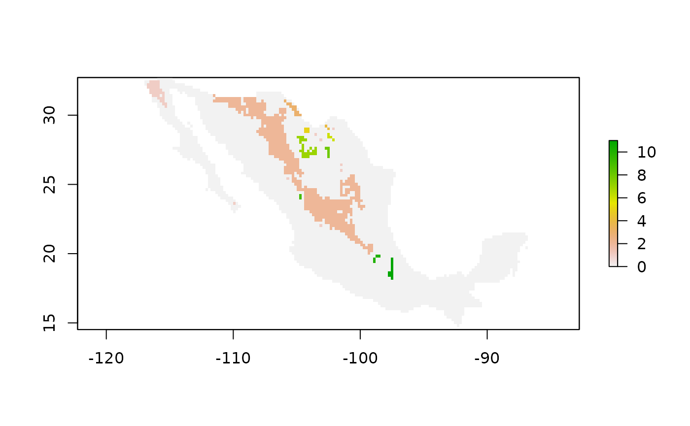
raster::plot(clustersin@raster_map)

Figure 3. An raster map showing the geographic clusters for a species that can travel two steps per unit time

The CSD diagram

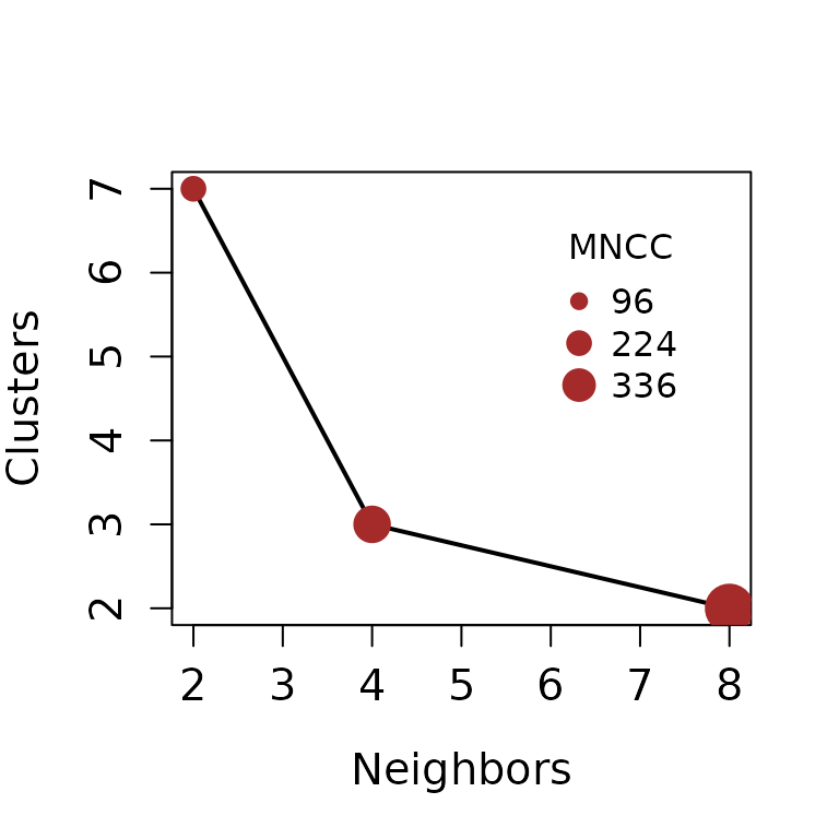
The CSD diagram is a simple but useful tool to estimate the number of dispersal steps that a species needs to travel per unit time in order to occupy its potential area of distribution. In this example the approximate number of dispersal steps to archive all suitable patches is 30 (not shown here).

csd_plot <- bamm::csd_estimate(sparse_mod,
                              dispersal_steps=c(2,4,8))
#>   |                                                                              |                                                                      |   0%  |                                                                              |=======================                                               |  33%  |                                                                              |===============================================                       |  67%  |                                                                              |======================================================================| 100%

Figure 4. Connectivity Sutitability Dispersal plot (CSD plot). The mean number of connected cells (MNCC) is showed in the legend.

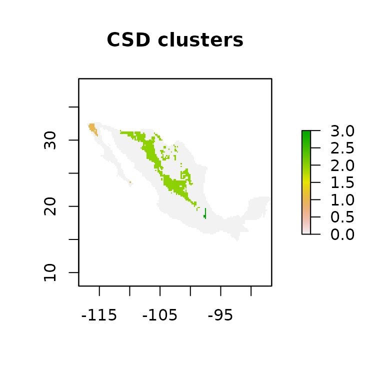
plot(csd_plot$csd$`dispersal_step:_4`@raster_map,
     main="CSD clusters")