Function to find the best n-dimensional ellipsoid model
Source:R/tenm_selection.R
tenm_selection.RdFinds the best n-dimensional ellipsoid model using a model calibration and selection protocol for ellipsoid models.
Usage
tenm_selection(
  this_species,
  omr_criteria = 0.1,
  ellipsoid_level = 0.975,
  vars2fit,
  nvars_to_fit = c(2, 3),
  mve = TRUE,
  proc = TRUE,
  sub_sample = TRUE,
  sub_sample_size = 1000,
  RandomPercent = 50,
  NoOfIteration = 1000,
  parallel = TRUE,
  n_cores = 4
)
Arguments
- this_species
An object of class sp.temporal.env representing species occurrence data organized by date. See
ex_by_date.- omr_criteria
Omission rate criterion used to select the best models. See
ellipsoid_selectionfor details- ellipsoid_level
Proportion of points to include inside the ellipsoid.
- vars2fit
A vector of variable names to use in building the models.
- nvars_to_fit
Number of variables used to build the models.
- mve
Logical. If
TRUE, a minimum volume ellipsoid will be computed.- proc
Logical. If
TRUE, compute the partial ROC test for each model.- sub_sample
Logical. Indicates whether to use a subsample of size sub_sample_size for computing pROC values, recommended for large datasets.
- sub_sample_size
Size of the sub_sample to use for computing pROC values when sub_sample is
TRUE.- RandomPercent
Percentage of occurrence points to sample randomly for bootstrap in the Partial ROC test. See
pROC.- NoOfIteration
Number of iterations for the bootstrap in the Partial ROC test. See
pROC.- parallel
Logical. Whether to run computations in parallel. Default is
TRUE.- n_cores
Number of cores to use for parallelization. Default is 4.
Value
An object of class "sp.temporal.selection" containing metadata of
model statistics of the calibrated models, obtainable from the "mods_table"
attribute. The function internally uses
ellipsoid_selection
to obtain model statistics. Note that this function inherits attributes
from classes "sp.temporal.modeling"
(see sp_temporal_data),
"sp.temporal.env" (see ex_by_date),
and "sp.temporal.bg" (see bg_by_date), thus all
information from these classes can be extracted from this object.
Examples
# \donttest{
library(tenm)
data("abronia")
tempora_layers_dir <- system.file("extdata/bio",package = "tenm")
abt <- tenm::sp_temporal_data(occs = abronia,
longitude = "decimalLongitude",
latitude = "decimalLatitude",
sp_date_var = "year",
occ_date_format="y",
layers_date_format= "y",
layers_by_date_dir = tempora_layers_dir,
layers_ext="*.tif$")
abtc <- tenm::clean_dup_by_date(abt,threshold = 10/60)
future::plan("multisession",workers=2)
abex <- tenm::ex_by_date(this_species = abtc,
train_prop=0.7)
abbg <- tenm::bg_by_date(abex,
buffer_ngbs=10,n_bg=50000)
future::plan("sequential")
varcorrs <- tenm::correlation_finder(environmental_data = abex$env_data[,-ncol(abex$env_data)],
method = "spearman",
threshold = 0.8,
verbose = FALSE)
#> Warning: the standard deviation is zero
vars2fit <- varcorrs$descriptors
mod_sel <- tenm::tenm_selection(this_species = abbg,
omr_criteria =0.1,
ellipsoid_level=0.975,
vars2fit = vars2fit,
nvars_to_fit=c(2,3),
proc = TRUE,
RandomPercent = 50,
NoOfIteration=1000,
parallel=TRUE,
n_cores=20)
#> -------------------------------------------------------------------
#> **** Starting model selection process ****
#> -------------------------------------------------------------------
#>
#> A total number of 36 models will be created for combinations of 9 variables taken by 2
#>
#> A total number of 84 models will be created for combinations of 9 variables taken by 3
#>
#> -------------------------------------------------------------------
#> **A total number of 120 models will be tested **
#>
#> -------------------------------------------------------------------
#> Doing calibration from model 1 to 40 in process 1
#>
#> Doing calibration from model 41 to 80 in process 2
#>
#> Doing calibration from model 81 to 120 in process 3
#>
#> Finishing calibration of models 1 to 40
#>
#> Finishing calibration of models 41 to 80
#>
#> Finishing calibration of models 81 to 120
#>
#> Finishing...
#>
#> -------------------------------------------------------------------
#> 82 models passed omr_criteria for train data
#> 17 models passed omr_criteria for test data
#> 17 models passed omr_criteria for train and test data
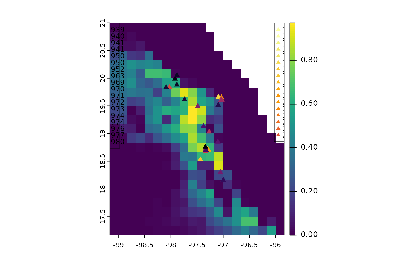
# Project potential distribution using bioclimatic layers for 1970-2000
# period.
layers_70_00_dir <- system.file("extdata/bio_1970_2000",package = "tenm")
suit_1970_2000 <- predict(mod_sel,model_variables = NULL,
layers_path = layers_70_00_dir,
layers_ext = ".tif$")
#> No selected variables. Using the first model in mods_table
#>
|
| | 0%
|
|======================================================================| 100%
terra::plot(suit_1970_2000)
colors <- c('#000004FF', '#040312FF', '#0B0725FF',
'#0B0725FF', '#160B38FF', '#160B38FF',
'#230C4CFF', '#310A5CFF', '#3F0966FF',
'#4D0D6CFF', '#5A116EFF', '#67166EFF',
'#741A6EFF', '#81206CFF', '#81206CFF',
'#8E2469FF', '#9B2964FF', '#A82E5FFF',
'#B53359FF', '#B53359FF', '#C03A50FF',
'#CC4248FF', '#D74B3FFF', '#E05536FF',
'#E9602CFF', '#EF6E21FF', '#F57B17FF',
'#F8890CFF', '#FB9806FF', '#FB9806FF',
'#FCA70DFF', '#FBB81DFF', '#F9C72FFF',
'#F9C72FFF', '#F6D847FF', '#F2E763FF',
'#F2E763FF', '#F3F585FF', '#FCFFA4FF',
'#FCFFA4FF')
points(abtc$temporal_df[,1:2],pch=17,cex=1,
col=rev(colors))
legend("topleft",legend = abtc$temporal_df$year[1:18],
col =rev(colors[1:18]),
cex=0.75,pch=17)
legend("topright",legend = unique(abtc$temporal_df$year[19:40]),
col = rev(colors[19:40]),
cex=0.75,pch=17)
 # }
# }