smop

The smop package is a small R package (it has four main functions) designed to perform the Mobility-Oriented Parity analysis (MOP) both in fast fashion and taking care of memory usage. To do this it uses optimized C++ code via the Rcpp and RcppArmadillo packages.

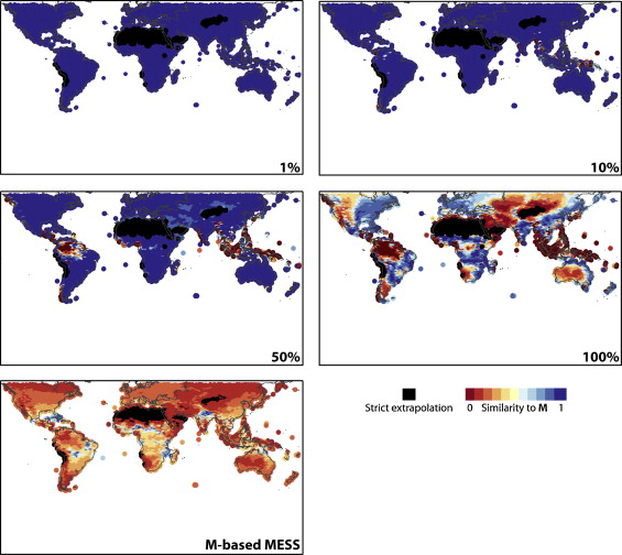
The MOP test was proposed in Owens et al. 2013 to estimate regions where extrapolation occurs (Figure 1).

Fig. 1. Extrapolation areas. Taken from Owens et al. 2013

Installation

You can install the development version of smop from GitHub with: remotes::install_github("luismurao/smop")

Example of use

First we estimate zones where strict extrapolation occurs. To show this, we read environmental data from the calibration and the transfer zones.

m_path <- system.file("extdata/M_layers", package = "smop") |>
                       list.files(full.names=TRUE)
g_path <- system.file("extdata/G_layers", package = "smop") |>
                       list.files(full.names=TRUE)
M_calibra <- terra::rast(m_path)
G_transfer <- terra::rast(g_path)

Calibration area

terra::plot(M_calibra)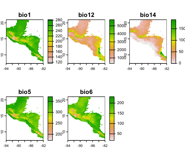

Fig. 2. Calibration area in Central America.

Model transfer area

terra::plot(G_transfer)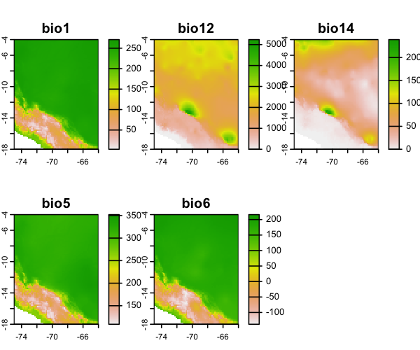

Fig. 3. Transfer area in South America.

Zones where strict extrapolation occurs.

extr_zones <- smop::extrapolation_zones(M_calibra = M_calibra,
                                        G_transfer = G_transfer,
                                        as_vec =FALSE)
terra::plot(extr_zones)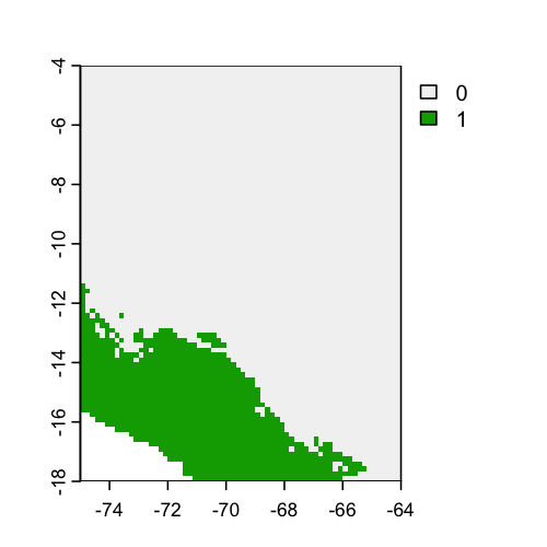

Fig. 4. Zones of strict extrapolation. The green zones represent areas where strict extrapolation occurs.

The MOP analysis

Now we perform the mop analysis

# Example 1 compute mop distance in serial
mop_test <- smop::mop(M_calibra = M_calibra, G_transfer =  G_transfer,
                      percent = 10,comp_each = NULL,
                      normalized = TRUE, standardize_vars=TRUE)
terra::plot(mop_test)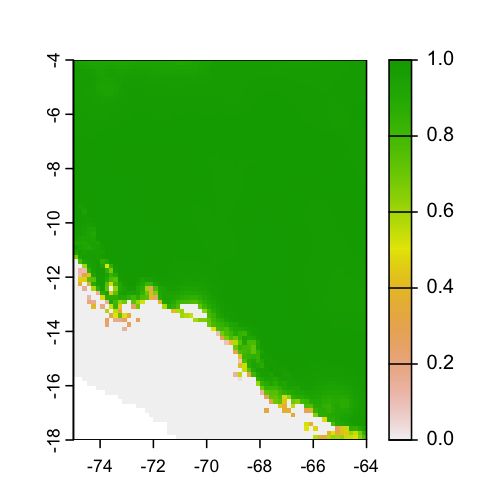

Fig. 5. MOP analysis. In this map zero values (in gray) represent zones of strict extrapolation and values above it are zones with analogous climates.

Parallel MOP

The MOP analysis can be performed in parallel by evoking functions from the furrr R package. Here, we use the comp_each parameter to specify the number of pixels to be processed in each CPU core. The number of pixels to be processed in each CPU core depends on the user’s RAM memory; if the user has a computer with few RAM, it is recommended to process by 500 pixels, otherwise, it can be as high as 10,000 pixels. An improvement from other versions of the mop function such as the ntbox and the kuenm, is that the performance of the function is less affected by the parametrization of the comp_each parameter.

# Example 2: Run the mop function in parallel
future::plan("future::multisession",workers = 2)
mop_test_parallel <- smop::mop(M_calibra = M_calibra,
                               G_transfer =  G_transfer,
                               percent = 10,comp_each = 500,
                               normalized = TRUE, standardize_vars=TRUE)
future::plan("future::sequential")
terra::plot(mop_test_parallel)

In fact, the better management of memory and the optimization of the code allows users to run MOP analyses on huge extents such as the whole world. Here, we show how to run the MOP using the bioclimatic variables for the current time at 10 arc minutes and an climate change scenario.

First, we downloaded the climatic layer for whole world for the current time at 10 arc minutes of resolution. Then, we downloaded the climate change layers at the same spatial resolution. Finally, we run the MOP analysis in a parallel fashion using 10 cores (MACBOOK PRO Apple M1 Max).

bio10_pre <- geodata::worldclim_global("bioc",res=10,path = tempdir())
bio10_fut <- geodata::cmip6_world("CNRM-CM6-1", "585", "2061-2080",
                              var="bioc", res=10, path=tempdir())

mop_time <- system.time({
  future::plan("future::multisession",workers = 10)
  mop_basic_res1 <- smop::mop(M_calibra = bio10_pre[[c(1,5,6,12,15)]],
                              G_transfer = bio10_fut[[c(1,5,6,12,15)]],
                              comp_each = 10000,
                              percent = 50,standardize_vars = TRUE,
                              normalized = TRUE)
  future::plan("future::sequential")
})

mop_time
#>     user   system  elapsed 
#>    47.362   5.575  748.391  

This process took about 12 minutes which seems to be a lot of time but note that this analysis was done for the whole world! Moreover, this kind of MOP analysis wont run on other packages.

Lets plot the result

terra::plot(mop_basic_res1)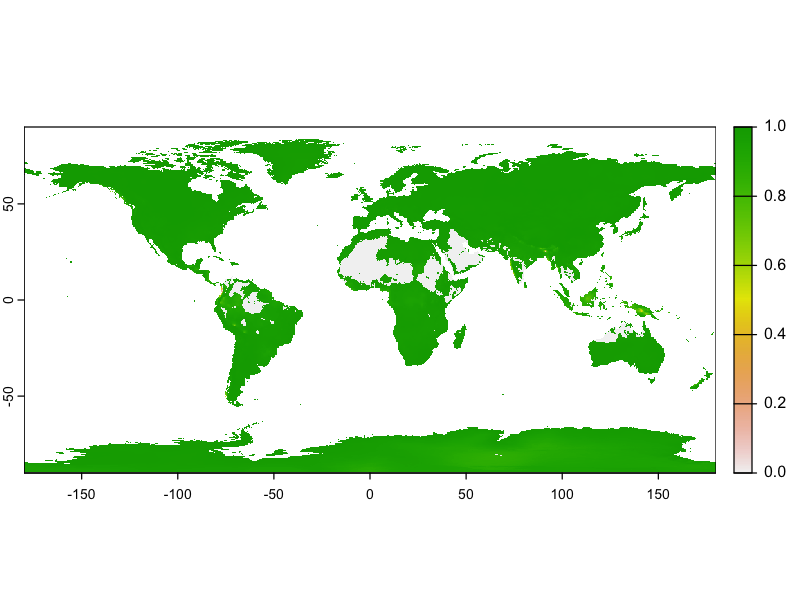

Fig. 6. MOP analysis for the whole world.

Acknowledgments

CONACYT Ciencia de Frontera CF-2023-I-1156. Laboratorio Nacional Conahcyt de Biología del Cambio Climático, México. To PAPIIT-UNAM IA202824 and PAPIIT-UNAM IA203922. RGCD thanks the Universidad Nacional Autónoma de México (Dirección General de Asuntos del Personal Académico, DGAPA-UNAM, México) for her postdoctoral scholarship.