ntbox: Reference guide, package version 0.5.1.4

Presentation

Here, we present a quick guide that will show the basics of the Graphical User Interface (GUI) of ntbox with the instructions of how to save the analysis in a workflow directory (at the end of this document); Note that the software is open-source, so you could see the code that it’s running behind the GUI by visiting the author’s github repository. You can find an improved version of this vignette in this web site https://luismurao.github.io/ntbox_user_guide.html

Launching the app

Load ntbox in your R session and type

library(ntbox)
run_ntbox()

First look

The above launches the Graphical User Interface (GUI) of ntbox

NicheToolBox GUI

ntbox sections

On navigation bar menu of the GUI, you will see 10 sections:

1. AppSettings: On this section you will specify three main inputs for your niche analysis:
   • Raster layers directory: this is the path to the directory where your niche layers are.
   • Projection layers directory: this is the path to the directory where your projection layers are.
   • Workflow directory: Path to the directory where ntbox results will be saved.
2. Data: The data section has methods to search and curate occurrence data. If the user does not have occurrence data, ntbox can download GBIF data via the spocc package; Data curation can be done via leaflet maps.
3. Niche Space: This provides methods extract and visualize information from the niche space (also called environmental space \(E\)).
4. Niche correlations: This section provides methods to visualize correlations and filter the environmental variables that are not correlated.
   
5. Niche clustering: Provides methods to perform k-means clustering and project the results in the geographic and environmental spaces (known as Hutchison’s duality (Colwell and Rangel 2009))
6. ENM: Methods to model the ecological niche; ntbox has functions to do bioclim (Busby, Margules, and Austin 1991; Booth et al. 2014) and ellipsoid models (Van Aelst and Rousseeuw 2009). Although the maxent (Phillips, Dudik, and Schapire 2004; Phillips and Dudík 2008) is not yet in the GUI interface, ntbox it could be run by using ntbox::maxent_callfunction on the command line.
7. SDM performance: Methods to measure the performance of the Species Distribution Models (SDM). These methods include Partial ROC (Peterson, Papes, and Soberon 2008), binomial tests (Anderson, Lew, and Peterson 2003), and the confusion matrix (Fielding and Bell 1997); also have map thresholding via several methodologies (Norris 2014; Jiménez-Valverde and Lobo 2007);
8. Extrapolation Risk: Methods to calculate environmental dissimilarity to evaluate extrapolation risk for model transfer exercises; it has Mobility-Oriented Parity (MOP) (Owens et al. 2013); Multivariate Environmental Similarity Surface (an optimized version) (Elith, Kearney, and Phillips 2010) and Exdet (Mesgaran, Cousens, and Webber 2014).
9. GIS Tools: Geographic Information System (GIS) tools to crop and mask raster layers and export them in other raster formats, make PCA transformation of the modeling layers.
10. Save state: By pressing the Save state button you can save the data and analysis that you have done inside the application.

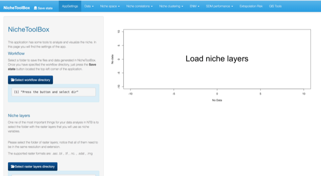
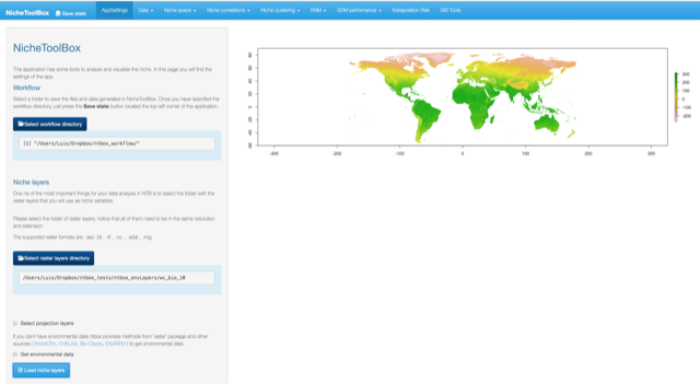
1. AppSettings configuring all you need

This section is one of the most important steps in the modeling process because here you are going to specify your workflow directory and also load or obtain the modeling layers.

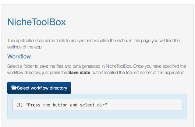
Workflow directory

This is a method that lets the user save the workflow of the ntbox session. It can be used once the user has specified the path to the directory where the workflow will be saved (on AppSettings section); Depending on what you have done this will create some subdirectories inside the workflow directory with the results of your analysis (a data table of the curated occurrence records in csv format, a heat map of the correlations between you niche variables, a leaflet map of the occurrence data, rasters of the geographic projection of the niche models, model evaluation results, etc.) and also will create an HTML document with a summary showing the code that was run on the GUI.

Please select workflow directory by pressing the button Select workflow directoy.

Workflow directory

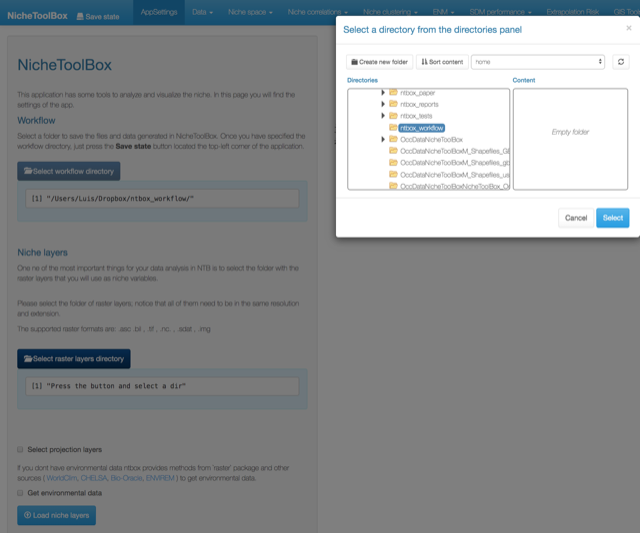
Select workflow directory

Go to Saving your analysis section for an example on how to save the things that you have done in your ntbox session.

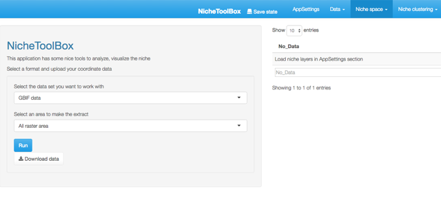
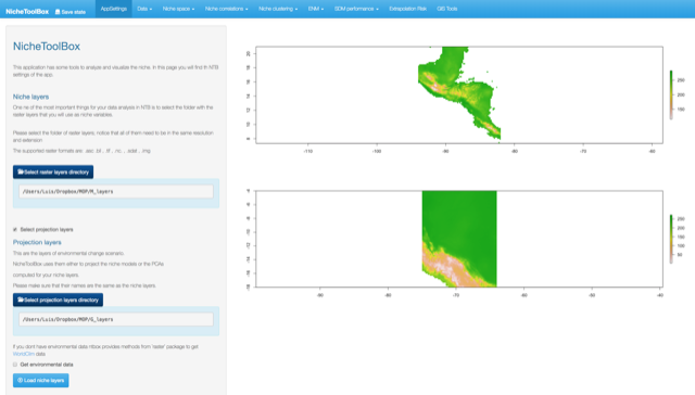
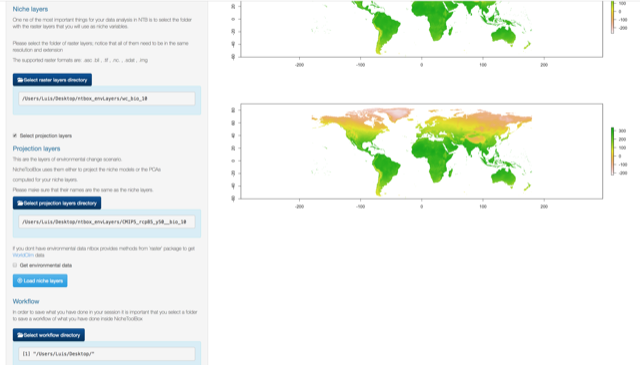
Uploading your niche layers

Go to the Niche layers section and click on select raster layers directory

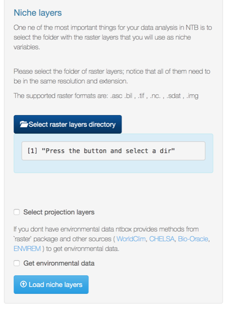
Niche layers directory

Once you have selected the directory click on Load niche layers button.

Load niche layers

Projection layers

These are the layers of environmental change (e.g. future or past) scenario(S). NicheToolBox uses them either to project the niche models or the PCAs computed for calibration layers; make sure that their names are the same as the niche layers.

Searching environmental data

Calibration layers

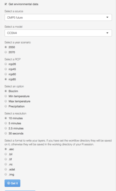
If you don’t have environmental layers, you can download them WorldClim data directly from ntbox by selecting the option Get envrionmental data; the available layers are:

• Bioclim (10, 5, 2.5 minutes; 30 secs)
• Min temperature (10, 5, 2.5 minutes; 30 secs)
• Max temperature (10, 5, 2.5 minutes; 30 secs)
• Precipitation (10, 5, 2.5 minutes; 30 secs)

Select the data you want to download and then press the Get button

Projection layers

Get IPPC5 climate projections from global climate models (GCMs) for four representative concentration pathways (RCPs) ( click here).

Aviable Global Climate Models

Select the data you want to download and then press the Get button

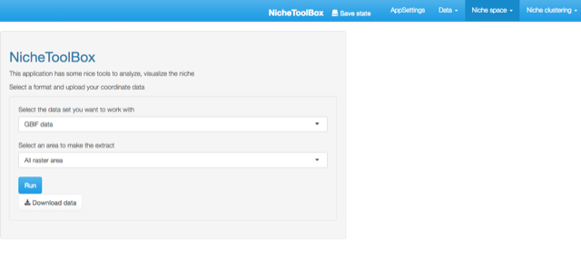
2. The Data section

ntbox can work with two sources of longitude/latitude data: a) GBIF records, which you can search, download and clean from GBIF, b) you can upload and clean your occurrence data from a local file.

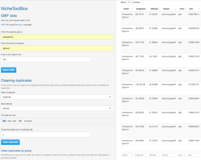
Searching GBIF records

Go to Data -> GBIF data. Enter species genus, species name where corresponds, and optionally specify the number of records that you want to search (occ search limit). Press Search GBIF button and wait. If the species is in the GBIF portal a data table will be displayed, if the species is not in GBIF, it will display the following message: “No occurrences found”.

In the next example we will search occurrence data for the species \(Ambystoma\,\,tigrinum\)

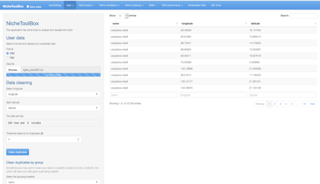
GBIF data cleaning

You can remove duplicate records using a separation (spatially filtering) distance in decimal degrees (default is 0). For Ambystoma tigrinum 480 records were downloaded before cleaning, and after clicking Clean duplicates with a \(\delta=0\) distance 154 remained, so there were 326 duplicate records.

GBIF search example

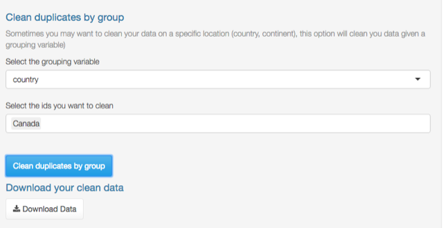
Clean duplicates by group

Suppose that your species has a huge geographic range and you want to work only with the records that match certain criteria, for example, records that lie within Canada. You can curate duplicate records using a grouping variable; in this example, the grouping variable must be country. Go to Clean duplicates by group section and select the grouping variable in this case country, then select the country (Canada) and click Clean duplicates by group.

Duplicate records

From 154 records only 2 are in Canada.

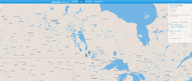
Duplicate records

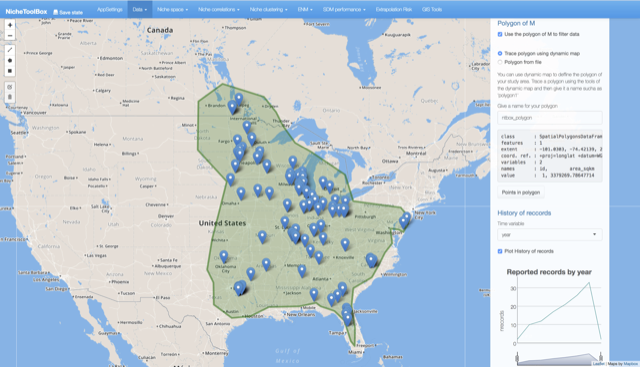
GBIF visualizations

The GBIF dataset has some fields that can be used to get some exciting visualizations, particularly fields related to observation date (year, month, day) and country. In Data -> GBIF data -> GBIF visualizations tab you can play with interactive plots, create animated visualizations and display a calendar of the reported records by year.

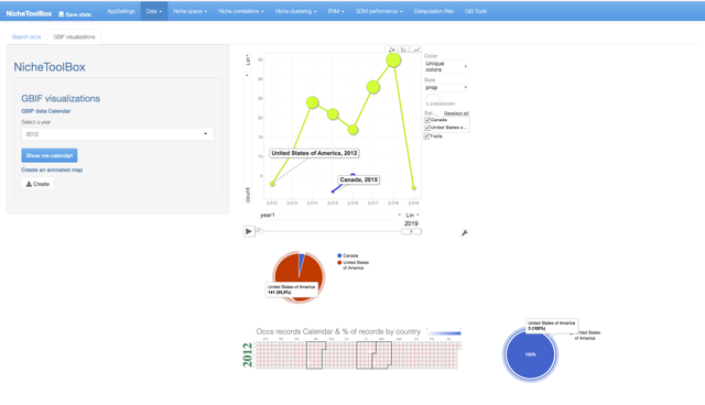
GBIF visualizations

GBIF visualizations

User data

You can use and clean your latitude and longitude data for the modeling process. Go to Data -> User data and upload your data. The data cleaning process is the same as the GBIF data.

User data

Geographic explorations using Dynamic Maps

We have seen how to curate data using threshold distances and grouping variables in ntbox. Now let’s see how to use leaflet maps to 1) display longitude/latitude data, 2) clean data and, 3) define our accessibility (or study) area or polygon (M data refers to the M concept from the BAM diagram conceptual framework, which in the niche modeling world is the accessible area where the species has been able to reach even if has not established; see Barve et al. (2011)(Barve et al. 2011) . for a broader explanation on this concept, 4) clean data using the M polygon. The above can be done for either the GBIF dataset or the User dataset.

Display longitude and latitude data

Go to Data -> Dynamic Map and on the right panel Select a dataset that you want to work with; in this case GBIF data will be used.

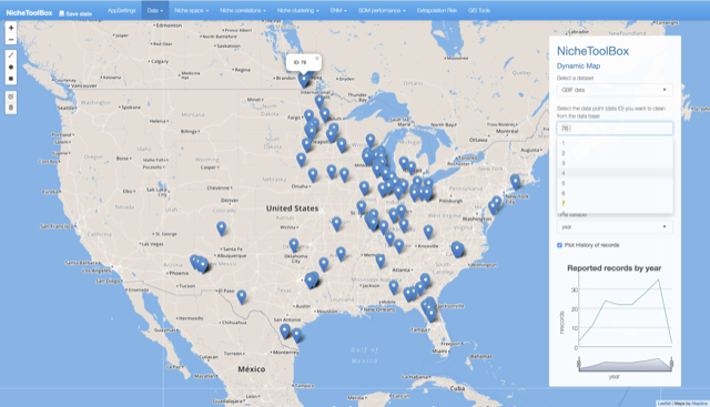
Dynamic map

Data curation using the Dynamic Map

On the right-side panel, there is an option where you can specify the data point id to remove it from the dataset. Click on the pop-up to see the point id, select it in the select input form from the right panel and press Clean data points button to clean.

Dynamic map

Define an M (accessibility area) polygon

You can use ntbox to define your study area. Go to Data -> Dynamic Map and in the right-side panel turn-on the button Define and work with M polygon, when activated you can either draw a polygon using the drawing tools (top-right corner) from ntbox or select your shapefile. If you prefer to define the M polygon using ntbox press the polygon tool and draw it:

Dynamic map polygon

Once defined, the polygon can be saved. In the right panel, there is a form where you can give a name for your polygon.

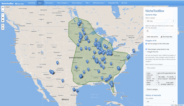
Dynamic map polygon

Data curation using the M polygon

We can filter the data points that lie inside the polygon. In the right panel just press the button Points in polygon

Polygon clean

3. Niche space

To work in Niche space (i.e., “environmental space”) we need to have loaded our niche raster layers (AppSettings “go to the first section of the tutorial”) and also a longitude/latitude dataset (GBIF data or User data).

1. Extracting niche values from raster layers

Go to Niche space -> Niche data extraction and select a longitude and latitude dataset. In the example, I selected the GBIF dataset. If the dataset is not empty and we have loaded the raster layers the app will not show any message:

Extract environmental data

On the contrary, if we have not loaded either the raster layers or the longitude/latitude data a message indicating what to do will be displayed.

When the dataset and the layers are in the app memory we can proceed to the next step. Here you just need to press the Run button and then a data table with the niche values of the longitude and latitude data will be displayed.

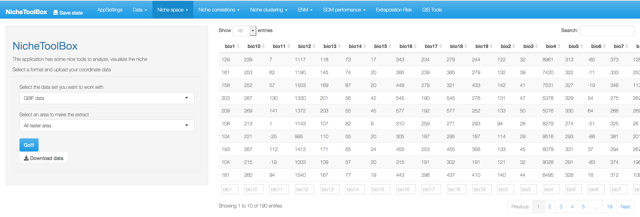
Extract environmental data

Niche explorations

We can explore our niche data using some exciting 3-Dimensional plots. Go to Niche space -> Known niche and play with \(x\), \(y\) and \(z\) variables of the ellipsoid plot.

Niche space

Niche trends

You can fit a (linear, quadratic, additive, smooth) model to see if your niche data have a trend.

Niche trends

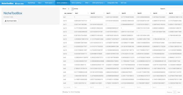
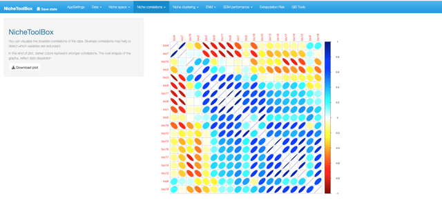
4. Niche correlations

One popular method to select the niche variables for modeling species niches and distributions is to study correlations among niche variables and filter those variables that are highly correlated. In Nichetoolbox you can filter the variables that summarize the environmental information of your presences (occurrences) data according to a correlation threshold; this algorithm suggests which variables to use for the modeling part.

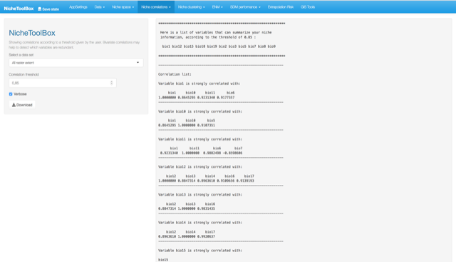
Niche correlations

Correlation matrix

Also, you can explore the correlation matrix and download it in .csv format.

Correlation matrix

Correlogram

Another thing that the user can do is to plot a correlogram.

Correlogram

5. Niche clustering

When studying species niches and distributions, one of the biggest questions that come to my mind is whether or not the species are adapting to different niche conditions. One way to explore this question is using clustering algorithms (a statistical tool which aims to observe if a multivariate dataset has a cluster structure in such a way that the data belonging to the same cluster are highly similar among them but different respect to other groups). If clusters are different, we can think that populations of the same species are responding in different ways to the same set of niche variables (i.e., they may be adapted to local conditions). However, think carefully about what you will conclude since many other processes could explain the observed pattern. This is just an exploratory tool.

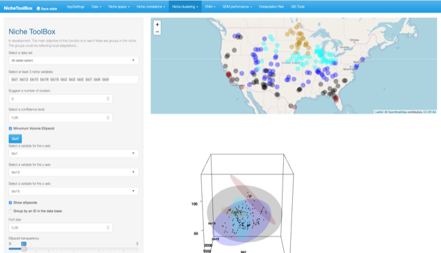
Go to Niche clustering -> K-means section and select at least 3 niche variables to make the cluster analysis. In my case, as I selected the bios of the WorldClim database as my niche layers, I used 19 niche variables, but if you want to work with fewer variables just delete some of them (Select at least 3 niche variables section).

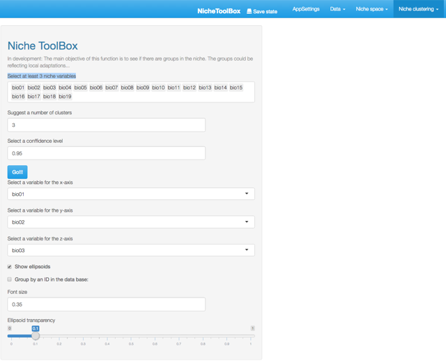
Niche clustering

Here it is necessary to indicate the number of clusters, the default value is 3 (in the future the app will have algorithms to help you to make this decision). Press the Go!!! button and you will see a 3-dimensional plot with ellipsoids representing the number of clusters you suggested. Bellow this plot you will see a leaflet map with the geographic projection of the points that fall inside each ellipsoid (colors help to identify to which cluster each data point belongs). his tool is designed to help you visualizing the Hutchison’s duality (Colwell and Rangel 2009).

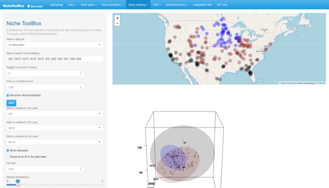
Niche clustering and visualization of the Hutchison’s duality

Let’s play with the number of clusters (now 5) and see how the results change…

Niche clustering and visualization of the Hutchison’s duality

6. ENM (Ecological niche modeling)

Ecological niche modeling (ENM), is a growing field in ecology and biogeography which aims to reconstruct the multidimensional ecological niche of species, from which to approximate its geographic distribution. ENM uses a set of mathematical and statistical tools to study the relationship between some environmental variables and species occurrences to estimate species niches and predict potential areas where the species can survive. These models have proved useful in ecology and conservation biology because they have been used to identify geographic localities that can be used to relocate endangered species, to study the impacts of climate change in biodiversity, to find biodiversity hotspots, vulnerability to invasive species and pathogens, among other applications (Peterson T. and Vieglais 2001; Peterson et al. 2011).

In Nichetoolbox you can model ecological niches by using one of the following modeling algorithms:

1. Minimum volume ellipsoid (Van Aelst and Rousseeuw 2009)
2. Bioclim (Booth et al. 2014)

Although the maxent (Phillips, Dudik, and Schapire 2004; Phillips and Dudík 2008) is not yet in the GUI interface, ntbox it could be run by using ntbox::maxent_callfunction on the command line.

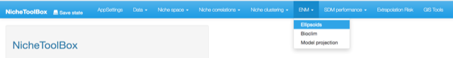
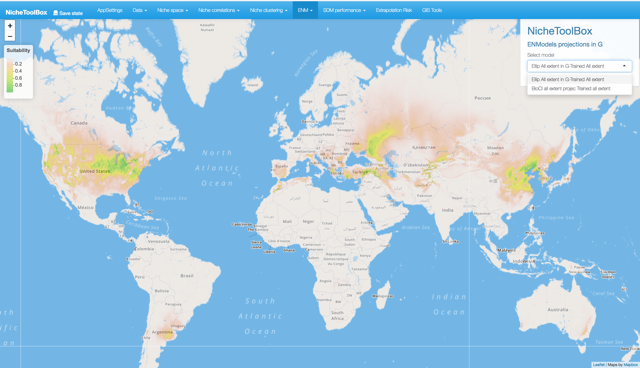
Ecological niche models

Minimum volume ellipsoid model

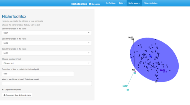
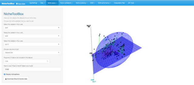
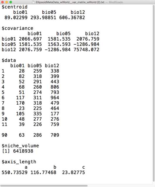
Ellipsoid models use the multinormal probability density function (PDF; equation 1) to compute the niche suitability index; the PDF is rescaled to have a suitability index defined in the interval \([0,1]\).

\[f\,(x_{1},x_{2},x_{3},..,x_{k})=\frac{1}{\left(2\pi\right)^{k}\mid\mathbf{\sum}\mid}\exp\left(-\frac{1}{2}\left(\mathbf{x-\mathbf{\mathbf{\mu}}}\right)^{\mathbf{T}}\mathbf{\sum}^{-1}\left(\mathbf{x-\mathbf{\mathbf{\mu}}}\right)\right)\,\,(1)\]

\[f\,(x_{1},x_{2},x_{3},..,x_{k})=1\,\exp\left(-\frac{1}{2}\left(\mathbf{x-\mathbf{\mathbf{\mu}}}\right)^{\mathbf{T}}\mathbf{\sum}^{-1}\left(\mathbf{x-\mathbf{\mathbf{\mu}}}\right)\right)\]

where \(\mathbf{x}\) is the vector of environmental variables such that each \(x_i\) represents an observation of the environmental variable \(i\). \(\Sigma\) is the covariance matrix of the occ data. \(\mu\) is the vector of means (centroids).

The \(({\mathbf x}-{\boldsymbol\mu})^\mathrm{T}{\boldsymbol\Sigma}^{-1}({\mathbf x}-{\boldsymbol\mu})\) is the square of the Mahalanobis distance.

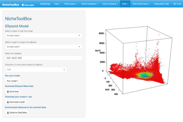
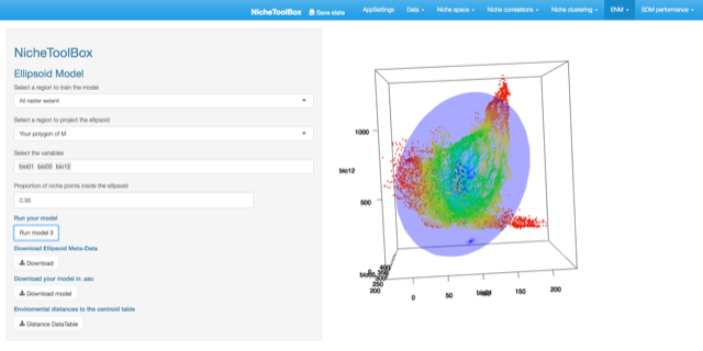
In Nichetoolbox, to make an ellipsoid model you just need the environmental information of your occurrence points and select which layers will define the axes of the niche model.

The model can be trained either with all occurrence data or with the occurrence points that lie inside your M polygon.

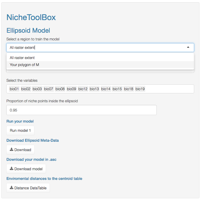
ENM M-polygon

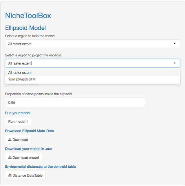
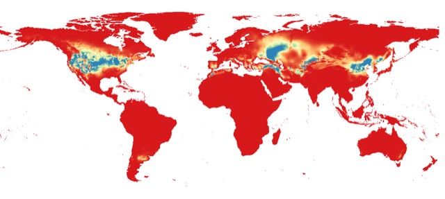
Similarly, you can project the model to the geography by using either the full extent of rasters or the extent of the M polygon.

Using full extent

ENM all extent

Select the niche variables and run your model.

Using the extent of the M polygon

Download ellipsoid meta-data.

Ellipsoid meta-data

Download the ellipsoid raster model.

Ellipsoid raster model

Download distance to the centroid table.

Distances to niche-centroid table

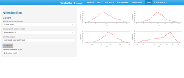
Bioclim model

The way that Bioclim model is implemented in Nichetoolbox is the same as the ellipsoid model:

• The model can be trained either with all occurrence data or with occurrence points that lie inside your M polygon.

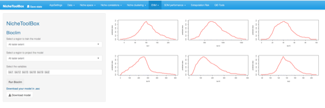
• Similarly, you can project the model to the geography using either the full extent of rasters or the extent of the M polygon.

ENM projection in geographic space

Once you have modeled your species’ niche using one or all modeling algorithms, you can explore them in geographic space by using the model visualizer. The visualizer is interactive (you can zoom in/out a map) and uses the leaflet library.

7. SDM performance

The last part of the project deals with species distribution model evaluation and performance. Nichetoolbox has two ways to evaluate models:

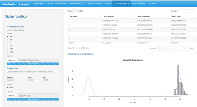
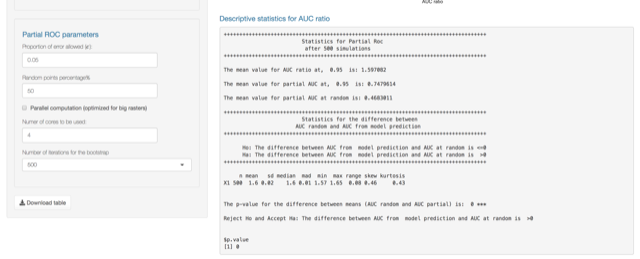
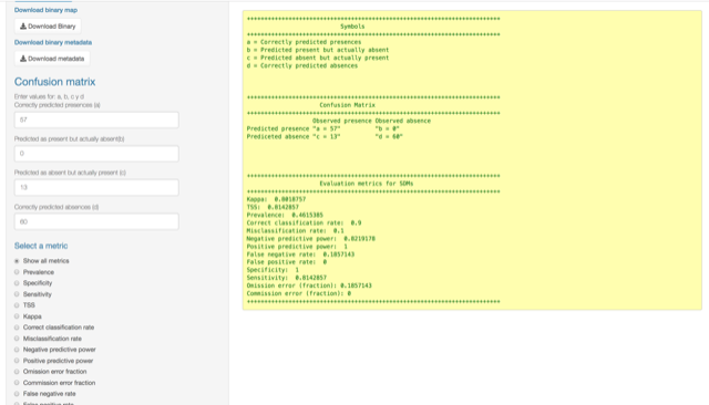
1. Partial Roc: This is a threshold independent technique proposed by (Peterson, Papes, and Soberon 2008) and it is also implemented on the kuenm package (Cobos et al. 2019).

2. Confusion matrix metrics: You can compute prevalence, specificity, sensitivity, TSS, Kappa, correct classification rate, misclassification rate, negative predictive power, positive predictive power, omission error fraction, commission error fraction, false negative rate, and false positive rate from the confusion metrics (Fielding and Bell 1997).

Partial ROC

To do Partial ROC analysis in Nichetoolbox upload your continuous niche model output map (e.g., from Maxent) and your validation dataset.

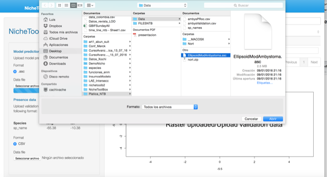
Validation data must be in the following format:

sp_name	longitude	latitude
Ambystoma tigrinum	-107.08333	51.08333
Ambystoma tigrinum	-102.41667	44.41667
Ambystoma tigrinum	-99.75000	45.91667
Ambystoma tigrinum	-85.75000	45.25000
Ambystoma tigrinum	-91.75000	45.75000
Ambystoma tigrinum	-91.41667	39.75000

Partial ROC output

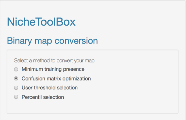
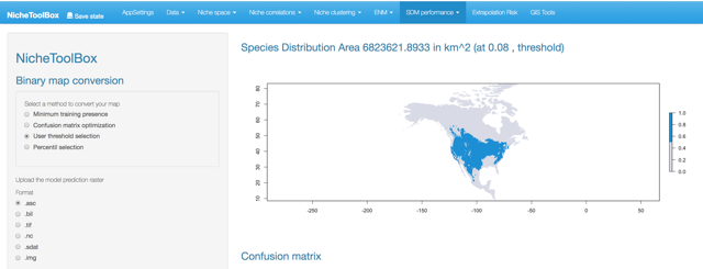
Binary maps

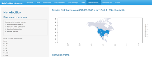
The ‘Binary maps’ section has functions to transform continuous models into binary maps (i.e., presence and absence of suitable conditions).

The conversion can be done by using one of the following methods:

• Minimum training presence: Uses the lowest suitability value where a presence occurs as a cut-off threshold.
• Confusion matrix optimization: By using true presences and absences the algorithm searches for the cut-off threshold that optimizes the value of Kappa and/or TSS statistic.
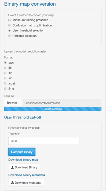
• User threshold selection: Uses the lowest suitability value where a presence occurs as a cut-off threshold.
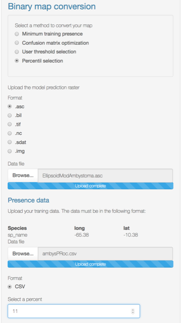
• Percent selection: The user can choose the percentile to make the cut-off. The 10 percentile is the default.

Minimum training presence

Just upload your continuous model (.asc) and your training data file (.csv).

Validation data must be in the following format:

	sp_name	longitude	latitude
85	Ambystoma tigrinum	-100.58333	31.91667
86	Ambystoma tigrinum	-91.08333	38.91667
87	Ambystoma tigrinum	-113.41667	42.75000
88	Ambystoma tigrinum	-121.41667	39.75000
89	Ambystoma tigrinum	-114.58333	42.91667
90	Ambystoma tigrinum	-94.41667	45.41667

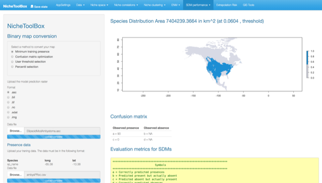
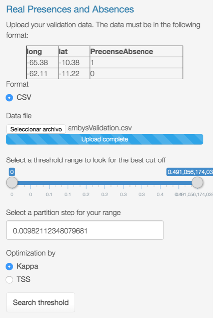
Confusion matrix optimization

The user uploads both the continuous map (.asc) and the presences/absences data file (.csv). The presences/absences data have to be in the following format:

longitude	latitude	presence_absence
-111.25000	36.91667	0
-106.20000	35.30000	1
-98.08000	47.74000	1
-93.27306	45.21076	1
-112.64406	36.58329	1
-101.85097	35.18559	1

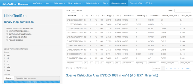
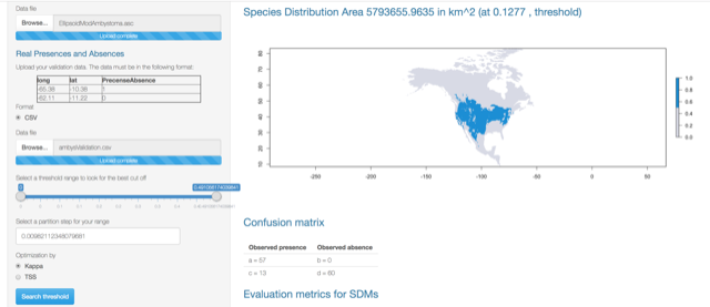
Once uploaded, press specify the range of thresholds to look for and press the Search threshold button.

The output looks like this:

User defined threshold

Specify a cut-off threshold.

The result is:

User defined threshold

Upload the continuous map and the presence data; then select the percentile that you want to work with (11 in this example).

The output is:

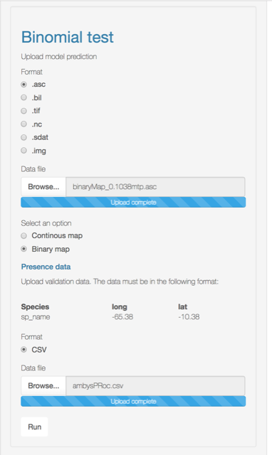
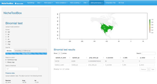
Binomial test

Compute the significance of a niche model by using the cumulative binomial probability of success of predicting correctly an occurrence given the validation data and the proportional area predicted as present in the niche model.

According to Anderson et al. (2003) (Anderson, Lew, and Peterson 2003), this test is “employed to determine whether test points fall into regions of predicted presence more often than expected by chance, given the proportion of map pixels predicted present by the model.”

You can upload your SDM model as a binary map or as a continuous model. If you choose the second, you will need to specify the threshold to convert it into a binary map.

8. Extrapolation risk (model uncertainty)

In this section you will find the tools to asses the extrapolation risk of the ecological niche models in a geographic context; this analysis becomes more important when doing model projections in time (e.g., climate change projections) or in geography (i.e., model transference from one calibration region to another region of interest).

The following analyses are available on ntbox:

• Mobility-Oriented Parity (MOP) (Owens et al. 2013)
• Multivariate Environmental Similarity Surfaces (MESS) (Elith, Kearney, and Phillips 2010)
• EXtrapolation DETection tool (ExDet) (Mesgaran, Cousens, and Webber 2014)

To do any of the analyses listed above use the environmental layers that you uploaded in the AppSettings section.

Mobility-Oriented Parity (MOP)

The MOP is calculated following Owens et al. (Owens et al. 2013).

1. Go to Extrapolation risk section and select MOP

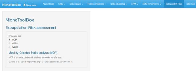
MOP

2. Select the variables that will be used to compute the MOP; these variables should be the same for both the M layers (the calibration layers of your niche model) and the G layers (projection layers).

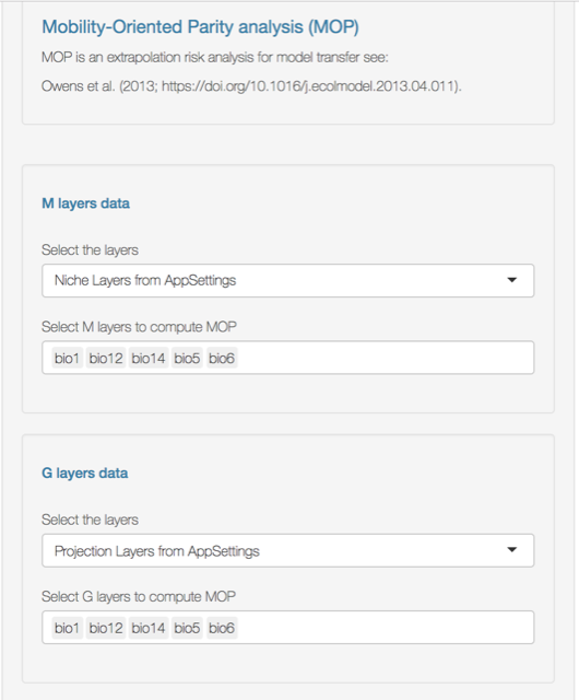
MOP

3. Select the percent of the reference points (i.e., pixels in M polygon layers) to be sampled (in this example 10%). You can also select the normalized version of MOP (normalized to 1 for regions that are more similar in both M and G regions). The computations can be done in parallel. This method is very efficient for big layers; the compute each parameter determines the number of pixels to be processed in each core (number of cores parameter).

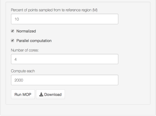
MOP

Press Run.

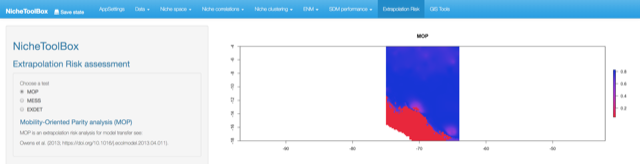
MOP

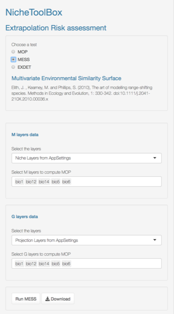
Multivariate Environmental Similarity Surfaces (MESS)

MESS is computed following (Elith, Kearney, and Phillips 2010). A version of this function is implemented in the dismo package (Hijmans et al. 2011) but the one in the ntbox package runs faster.

As in MOP, you need to select which variables will be used to compute the MESS and then press the Run button.

MESS

The result is:

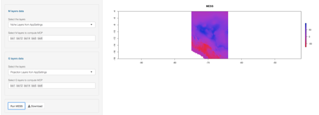
MESS

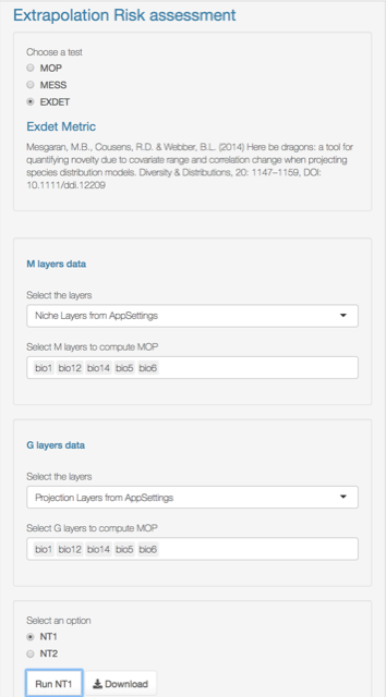
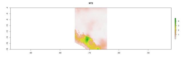
Extrapolation Detection tool (ExDet)

Exdet means “Extrapolation Detection tool” and it is computed following (Mesgaran, Cousens, and Webber 2014). In https://www.climond.org/ExDet.aspx the authors mention that

The ExDet tool, based on the Mahalanobis distance measures the similarity between reference and projection domains by accounting for both the deviation from the mean and the correlation between variables. In ntbox you can do the two types of ExDet analysis:

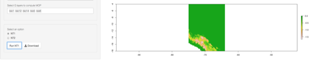
1. NT1 (univariate extrapolation)
2. NT2 (multivariate extrapolation)

NT1

Select the Exdet in the left panel of ntbox, then select which variables are going to be used in the analysis for the M and G region.

Exdet NT1

Press run and the result looks like this:

Exdet NT1

NT2

Follow the above steps and you will see:

Exdet NT2

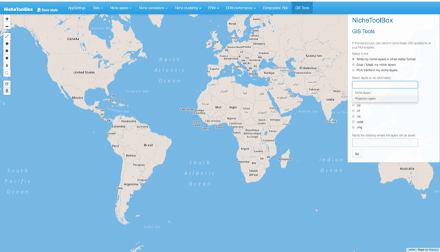
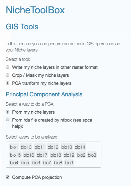
9. GIS tools

Here we provide methods to do some Geographic Information System (GIS) operations. In the GIS tools section you can do the following:

• Export your environmental layers into other formats: this is very useful as some of the ecological niche modeling software use as input a specific format for the environmental data (e.g. .asc format in maxent).
• Crop or mask the environmental layers: Crop or mask the environmental layer given a polygon defined by the user.
• Principal component transformation: Make a principal component analysis (PCA) of your environmental layers and make the spatial/temporal projection of them.

To do any of the analyses listed above, upload your environmental layers in the AppSettings section and set your working directory.

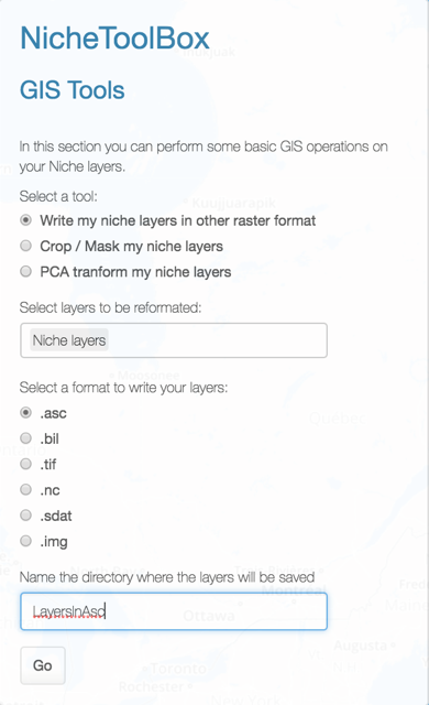
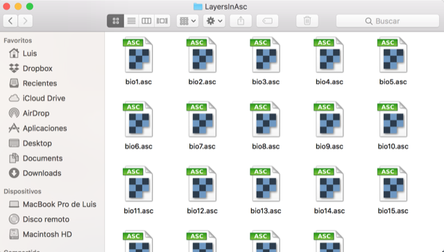
Export your environmental layers into other formats

Just select which layers to export into one of the available formats.

• .asc
• .bil
• .tif
• .nc
• .sdat
• .img

Give a name to the folder where they will be exported and press go.

The output is:

Crop or mask the environmental layers

In the GIS tools section, you can create a polygon of your M (calibration) and G (projection) regions to crop or mask the environmental layers that will be used in the modeling process.

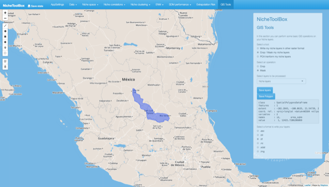
Select the format to export the crop/masked layers

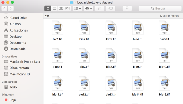
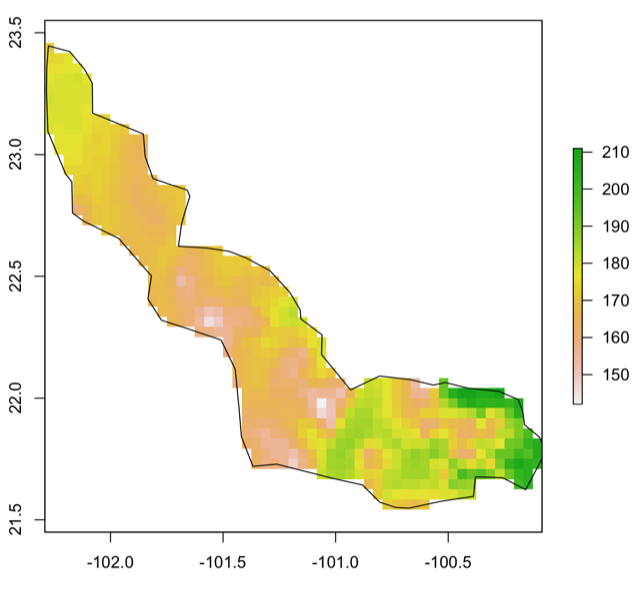
ntbox will create a folder called ntbox_nicheLayersMasked

This is the visualization of the masked layers

Principal component transformation

You can do a principal components analysis (PCA) of your environmental layers and project them in time or space. As in all the analysis of this section, you should upload your environmental layers in the AppSettings section and set your working directory.

The transformation can be computed on the flight (the option From my niche layers) or in a previous ntbox session by using the rda file (see the help of the function ?ntbox::spca).

To do the PCA transformation and project it, you must ensure that both the calibration layers and projection layers are listed in the same order (or named equal). This means that if you have a set of calibration layers called bio1, bio2, bio6, and bio12, the projection layers will need to be in the same order cc85bi501, cc85bi502, cc85bi506, cc85bi5012.

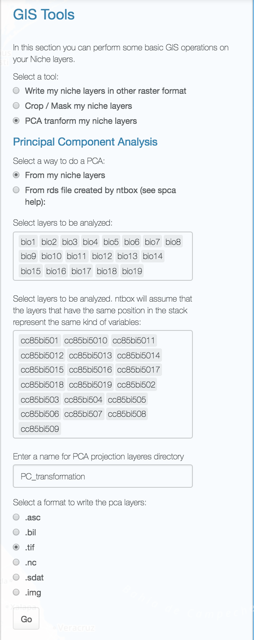
Just select a format for your PC layers and give a name to the directory where they will be saved. When the computation is done you will see a scree plot of the explained variance by each component.

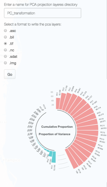
The above will create 2 folders, pca_referenceLayers for the calibration layers and PC_projection for the calibration.

10. Saving your analysis

Your analysis can be saved just by pressing the Save state button located in the top-left corner of the application.

It is worth noting that you can save your analysis at any stage of the workflow. Depending on the analysis performed, you will find a directory with the results of each analysis, for example:

• ntbox_envLayers: A directory created for the environmental information downloaded directly from ntbox (WorldClim, ENVIREM, Bio-Oracle, CHELSA).
• ntbox_OccData: Occurrence data files (the raw data from GBIF, the user data, the data cleaned using the spatial filter or/and the dynamic map).
• ntbox_NicheData: Niche data files (the environmental values of occurrence data, correlation results, k-means clustering results).
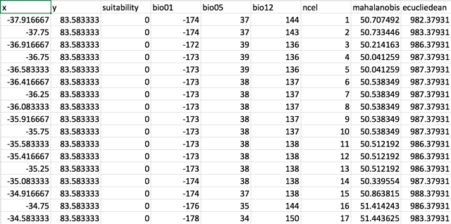
• ntbox_enm_files: Ecological niche modeling results (geographic projection files in .asc format for ellipsoids and bioclim models).
• ntbox_model_eval_files: Model evaluation files (partial ROC results, binomial test results, map binarization results -confusion matrix optimization, minimum training presence, etc-).
• ntbox_extrapolation_risk_files: Extrapolation risk assessment files (MOP, MESS and Exdet results in raster format).
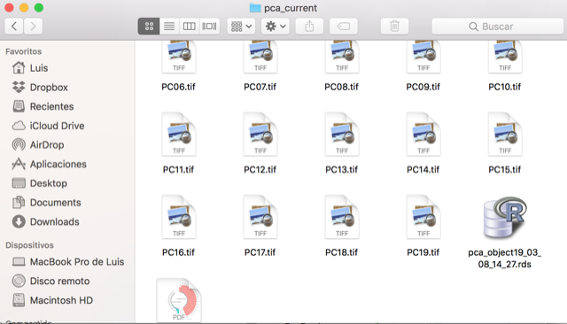
• GIS tools results: Principal Components raster files, PCs transfers in time or space, cropped and masked layers.
• ntbox_workflowReport: These are HTML files with the code that ntbox used to generate the analysis and results inside the graphical user interface (data_report.html, niche_data_report.html, enm_report.html, model_eval_report.htm, and extrapolation_risk_report.html). The figure below shows some of these files.

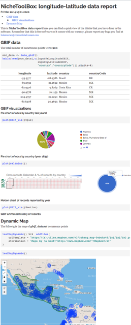
ntbox_10_gdata.html

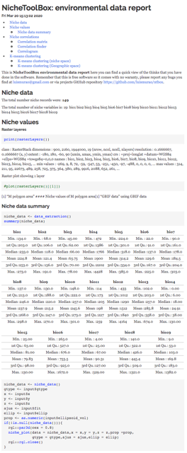
ntbox_10_env_data.html

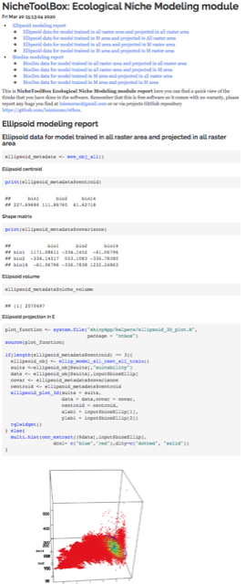
ntbox_10_enm.html

ntbox_10_enm_eval.html

References

Anderson, R P, D Lew, and A Townsend Peterson. 2003. “Evaluating predictive models of species’ distributions: Criteria for selecting optimal models.” Ecol. Model. 162: 211–32.

Barve, Narayani, Vijay Barve, Alberto Jiménez-Valverde, Andrés Lira-Noriega, Sean P. Maher, a. Townsend Peterson, Jorge Soberón, and Fabricio Villalobos. 2011. “The crucial role of the accessible area in ecological niche modeling and species distribution modeling.” Ecol. Modell. 222 (11): 1810–9. https://doi.org/10.1016/j.ecolmodel.2011.02.011.

Booth, Trevor H., Henry A. Nix, John R. Busby, and Michael F. Hutchinson. 2014. “bioclim: the first species distribution modelling package, its early applications and relevance to most current MaxEnt studies.” Edited by Janet Franklin. Divers. Distrib. 20 (1): 1–9. https://doi.org/10.1111/ddi.12144.

Busby, J R, C R Margules, and M P Austin. 1991. “BIOCLIM - A bioclimate analysis and prediction system.” In Nat. Conserv. Cost-Effective Biol. Surv. Data Anal., edited by C R Margules and M P Austin, 64. Canberra, Australia.

Cobos, Marlon E., A. Townsend Peterson, Narayani Barve, and Luis Osorio-Olvera. 2019. “Kuenm: An R Package for Detailed Development of Ecological Niche Models Using Maxent.” PeerJ 7 (February): e6281. https://doi.org/10.7717/peerj.6281.

Colwell, Robert K., and Thiago F. Rangel. 2009. “Hutchinson’s duality: The once and future niche.” Proc. Natl. Acad. Sci. USA 106 (2): 19651–8. https://doi.org/10.1073/pnas.0901650106.

Elith, Jane, Michael Kearney, and Steven Phillips. 2010. “The art of modelling range-shifting species.” Methods Ecol. Evol. 1 (4): 330–42.

Fielding, Alan H., and John. Bell. 1997. “A review of methods for the assessment of prediction errors in conservation presence/absence models.” Environ. Conserv. 24 (1): 38–49.

Hijmans, R J, S Phillips, J Leathwick, and J Elith. 2011. “Package dismo: Species distribution modeling.” http://cran.r-project.org/web/packages/dismo/index.html.

Jiménez-Valverde, Alberto, and Jorge M. Lobo. 2007. “Threshold criteria for conversion of probability of species presence to either-or presence-absence.” Acta Oecologica 31: 361–69. https://doi.org/10.1016/j.actao.2007.02.001.

Mesgaran, Mohsen B., Roger D. Cousens, and Bruce L. Webber. 2014. “Here be dragons: a tool for quantifying novelty due to covariate range and correlation change when projecting species distribution models.” Edited by Janet Franklin. Divers. Distrib. 20 (10): 1147–59. https://doi.org/10.1111/ddi.12209.

Norris, Darren. 2014. “Model thresholds are more important than presence location type: Understanding the distribution of lowland tapir (Tapirus terrestris) in a continuous Atlantic forest of southeast Brazil.” Trop. Conserv. Sci. 7 (3): 529–47. https://doi.org/10.1177/194008291400700311.

Owens, Hannah L, Lindsay P Campbell, L Lynnette Dornak, Erin E Saupe, Narayani Barve, Jorge Soberón, Kate Ingenloff, et al. 2013. “Constraints on interpretation of ecological niche models by limited environmental ranges on calibration areas.” Ecol. Modell. 263 (0): 10–18. https://doi.org/http://dx.doi.org/10.1016/j.ecolmodel.2013.04.011.

Peterson, A. Townsend, Monica Papes, and Jorge Soberon. 2008. “Rethinking receiver operating characteristic analysis applications in ecological niche modeling.” Ecol. Modell. 213 (1): 63–72.

Peterson, A. Townsend, Jorge Soberón, Richard G Pearson, Robert P Anderson, E Martínez-Meyer, Miguel Nakamura, and Miguel Bastos Araujo. 2011. Ecological niches and geographic distributions. Princeton University Press. https://doi.org/10.5860/CHOICE.49-6266.

Peterson T., A, and David Vieglais. 2001. “Predicting species invasions using ecological niche modeling.” Bioscience 51: 363–71.

Phillips, S, M Dudik, and R Schapire. 2004. “A maximum entropy approach to species distribution modeling.” In 21st Int. Conf. Mach. Learn. Banff, Canada.

Phillips, Steven J., and Miroslav Dudík. 2008. “Modeling of species distributions with Maxent: New extensions and a comprehensive evaluation.” Ecography (Cop.). 31 (2): 161–75.

Van Aelst, Stefan, and Peter Rousseeuw. 2009. “Minimum volume ellipsoid.” Wiley Interdiscip. Rev. Comput. Stat. 1 (1): 71–82. https://doi.org/10.1002/wics.19.