An introduction to ellipsoid model selection
Source:vignettes/ellipsoid_selection.Rmd
ellipsoid_selection.Rmdlibrary(ntbox)
We demonstrate the use of the model selection protocol implemented in ntbox by using occurrence data for the giant hummingbird (Patagona gigas). The occurrence records and the modeling layers are available in the ntbox package (if you haven’t installed it go to this link where you will find the installation notes for each of the operating systems).

Fig. 1 Patagona gigas taken from wikimedia
Loading the occurrence data
With the following commands, you can load into your R session the geographic records
# Occurrence data for the giant hummingbird (Patagona gigas)
pg <- utils::read.csv(system.file("extdata/p_gigas.csv",
                                  package = "ntbox"))

head(pg)
#>          species longitude   latitude  type
#> 1 Patagona gigas -65.21600 -22.790906 train
#> 2 Patagona gigas -78.32320  -0.459242  test
#> 3 Patagona gigas -68.06772 -16.538205 train
#> 4 Patagona gigas -70.51691 -33.385099 train
#> 5 Patagona gigas -70.31293 -33.352039 train
#> 6 Patagona gigas -70.58427 -34.274945  test
As you can see in the table there are 4 columns: “species”, “longitude” and “latitude” and “type” (with train or test as factors). The data points with the train labels are going to be used for model calibration and the test points will be used for selection.
Bioclimatic layers
Let’s load the environmental information and display it
# Bioclimatic layers path
wcpath <- list.files(system.file("extdata/bios",
                                package = "ntbox"),
                    pattern = ".tif$",full.names = TRUE)

wc <- raster::stack(wcpath)

plot(wc[[1]])
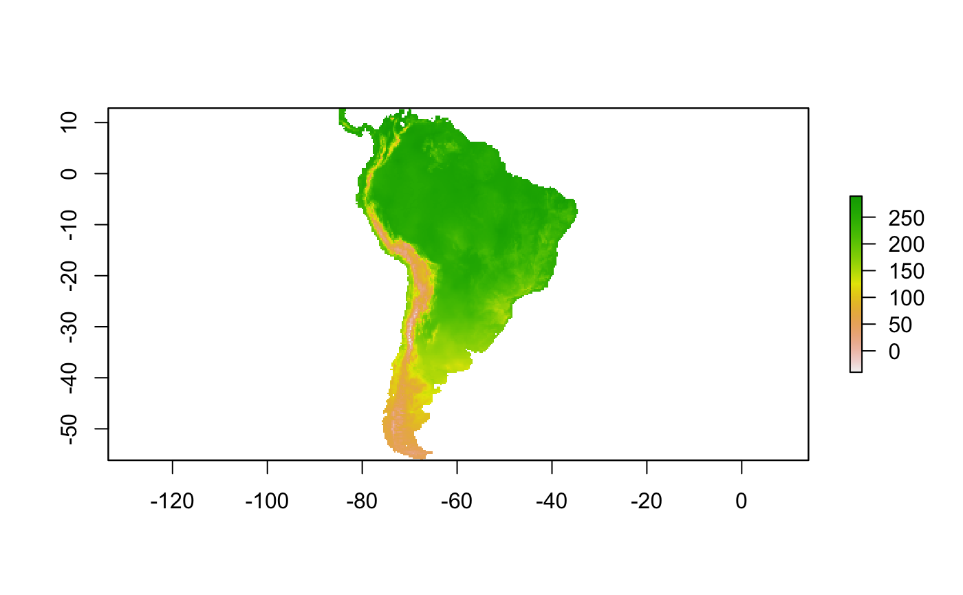
The environmental information is for South America and here we will project our niche model …
Split occurrence
Now we split the occurrence data into train and test using the type variable; the choice of the data is normally done using different partition methods, but in our case, the data previously was split using a random partition.
# Split occs in train and test
pgL <- base::split(pg,pg$type)
pg_train <- pgL$train
pg_test <- pgL$test
Extract the environmental information
The following code extracts the environmental information for both train and test data
pg_etrain <- raster::extract(wc,pg_train[,c("longitude",
                                            "latitude")],
                             df=TRUE)
pg_etrain <- pg_etrain[,-1]

head(pg_etrain)
#>    bio01  bio02 bio03   bio04  bio05  bio06  bio07  bio08  bio09  bio10 bio11
#> 1  82.80 193.68 62.16 4088.88 219.60 -90.00 309.60 123.96  25.80 123.96 23.56
#> 2  50.20 145.80 69.60 1523.60 145.40 -62.80 208.20  61.20  28.40  65.20 27.40
#> 3  94.76 147.56 56.80 4035.48 238.52 -17.76 256.28  51.08 146.36 146.36 43.08
#> 4  54.08 139.56 56.84 3963.12 189.68 -53.04 242.72   7.12 104.52 104.52  4.04
#> 5 149.24 135.32 53.64 4122.48 290.08  39.68 250.40 101.72 200.44 202.60 96.08
#> 6 111.20 140.00 54.00 4233.40 266.20   8.80 257.40  64.60 161.20 168.60 58.20
#>     bio12  bio13 bio14  bio15  bio16 bio17  bio18  bio19
#> 1  249.52  65.28  0.00 108.68 172.56  2.96 172.56   3.92
#> 2  605.20 129.00  6.00  77.00 325.20 29.20 191.40  29.20
#> 3  571.20 128.80  3.64  91.88 337.48 16.64  16.64 327.20
#> 4  469.68 108.20  3.76  88.68 267.28 18.48  18.48 261.48
#> 5  424.84 109.32  1.36 105.16 278.00  9.80   9.80 269.96
#> 6 1340.80 279.80 18.20  82.80 766.80 68.20  71.80 701.60

pg_etest <- raster::extract(wc,pg_test[,c("longitude",
                                          "latitude")],
                            df=TRUE)
pg_etest <- pg_etest[,-1]

head(pg_etest)
#>    bio01  bio02 bio03   bio04  bio05 bio06  bio07  bio08  bio09  bio10  bio11
#> 1  56.96  84.56 83.36  500.52 112.08 11.48 100.60  56.80  53.80  60.96  49.48
#> 2 108.80 140.20 53.20 4359.80 258.80 -2.00 260.80  59.40 160.20 165.80  53.60
#> 3 138.00 106.00 63.00 2240.00 231.00 63.00 168.00 109.00 164.00 168.00 109.00
#> 4 135.36 128.16 59.24 3250.52 255.56 40.28 215.28  93.84 176.84 176.92  92.84
#> 5 161.80 106.60 53.20 3360.20 273.60 73.80 199.80 123.80 204.80 204.80 118.80
#> 6 136.88 119.04 53.20 3559.80 265.56 43.24 222.32  98.64 178.72 183.88  91.04
#>     bio12  bio13 bio14  bio15  bio16  bio17  bio18  bio19
#> 1 1223.80 128.04 70.00  16.56 364.88 243.44 307.56 286.68
#> 2  840.20 194.00  3.80  95.80 522.00  20.20  21.80 483.20
#> 3  349.00  95.00  0.00 111.00 239.00   3.00   3.00 239.00
#> 4  498.08 136.56  1.36 108.64 331.80   7.32   7.32 331.52
#> 5  504.40 130.60  2.40 103.40 331.20   9.60   9.60 312.80
#> 6  835.56 201.76  3.16  99.88 533.76  15.96  21.60 508.16
Specify the number of variables to fit the model
Now we specify the number of variables to fit the ellipsoid models; in the example, we will fit for 3,5, and 6 dimensions
nvarstest <- c(3,5,6)
The level parameter
This parameter is to specify the proportion of training points that will be used to fit the minimum volume ellipsoid (Van Aelst and Rousseeuw 2009).
# Level
level <- 0.99
Environmental background to compute the approximated AUC ratio
This background data is just to compute the partial ROC test
env_bg <- ntbox::sample_envbg(wc,10000)
Set the omission rate criteria
For selecting the model we will use an arbitrary value of 6 percent of omission; it is not a rule but accepted omission rates are those bellow 10%. We will ask the function to return the partial ROC value (Peterson, Papes, and Soberon 2008)
omr_criteria <- 0.06
proc <- TRUE
Model calibration and selection protocol
To calibrate the models ntbox estimates all combinations (\(C^n_k\)) of \(n\) variables, taken \(k\) at a time for each \(k= 2,3,\dots, m\), where \(m\) is lesser than \(n\). It is known that
\[\displaystyle C^n_k =\frac {n!}{k!(n-k)!}.\]
Now we just need to use the function ellipsoid_selection to run the model calibration and selection protocol.
e_selct <- ntbox::ellipsoid_selection(env_train = pg_etrain,
                                      env_test = pg_etest,
                                      env_vars = env_vars,
                                      level = level,
                                      nvarstest = nvarstest,
                                      env_bg = env_bg,
                                      omr_criteria= omr_criteria,
                                      proc = proc)
#> -----------------------------------------------------------------------------------------
#>      **** Starting model selection process ****
#> -----------------------------------------------------------------------------------------
#>
#> A total number of 35 models will be created for combinations of 7 variables taken by 3
#>
#> A total number of 21 models will be created for combinations of 7 variables taken by 5
#>
#> A total number of 7 models will be created for combinations of 7 variables taken by 6
#>
#> -----------------------------------------------------------------------------------------
#>   **A total number of 63 models will be tested **
#>
#> -----------------------------------------------------------------------------------------
#>   5 models passed omr_criteria for train data
#>   5 models passed omr_criteria for test data
#>   2 models passed omr_criteria for train and test data
Let’s see the first 20 rows of the results
head(e_selct,20)
#>                            fitted_vars nvars om_rate_train om_rate_test
#> 1                    bio01,bio02,bio07     3    0.04201681   0.03921569
#> 2                    bio01,bio02,bio03     3    0.05882353   0.05882353
#> 3                    bio01,bio07,bio12     3    0.06722689   0.05882353
#> 4                    bio01,bio02,bio12     3    0.06722689   0.05882353
#> 5                    bio01,bio02,bio18     3    0.05882353   0.07843137
#> 6                    bio01,bio03,bio07     3    0.06722689   0.07843137
#> 7                    bio01,bio03,bio12     3    0.09243697   0.05882353
#> 8                    bio01,bio12,bio18     3    0.07563025   0.07843137
#> 9                    bio07,bio12,bio18     3    0.05882353   0.09803922
#> 10                   bio01,bio03,bio18     3    0.09243697   0.07843137
#> 11                   bio02,bio12,bio18     3    0.07563025   0.09803922
#> 12                   bio02,bio07,bio18     3    0.07563025   0.09803922
#> 13                   bio01,bio07,bio18     3    0.08403361   0.09803922
#> 14                   bio02,bio03,bio18     3    0.06722689   0.11764706
#> 15                   bio03,bio07,bio18     3    0.06722689   0.11764706
#> 16                   bio12,bio18,bio19     3    0.05882353   0.13725490
#> 17 bio01,bio02,bio03,bio07,bio12,bio18     6    0.10924370   0.09803922
#> 18       bio01,bio03,bio12,bio18,bio19     5    0.10084034   0.11764706
#> 19                   bio02,bio03,bio07     3    0.14285714   0.07843137
#> 20       bio01,bio02,bio03,bio07,bio12     5    0.12605042   0.09803922
#>    bg_prevalence     pval_bin pval_proc env_bg_paucratio env_bg_auc
#> 1     0.16997727 0.000000e+00         0         1.684529  0.9404397
#> 2     0.23609052 0.000000e+00         0         1.626512  0.9313332
#> 3     0.16859373 0.000000e+00         0         1.741612  0.9413885
#> 4     0.19903152 0.000000e+00         0         1.663874  0.9226301
#> 5     0.19626445 0.000000e+00         0         1.659621  0.9112729
#> 6     0.21276806 0.000000e+00         0         1.628072  0.9328180
#> 7     0.16681490 0.000000e+00         0         1.711789  0.9403048
#> 8     0.20189742 0.000000e+00         0         1.659902  0.8984794
#> 9     0.40260895 9.103829e-15         0         1.388005  0.8266110
#> 10    0.15406661 0.000000e+00         0         1.746153  0.9404541
#> 11    0.39243008 2.886580e-15         0         1.408482  0.7819235
#> 12    0.40962546 1.953993e-14         0         1.320024  0.8184062
#> 13    0.17808084 0.000000e+00         0         1.691070  0.9304089
#> 14    0.41328194 3.923528e-13         0         1.306047  0.8177104
#> 15    0.42761142 1.670664e-12         0         1.263668  0.8103704
#> 16    0.37296176 6.283862e-14         0         1.388973  0.7452276
#> 17    0.08716276 0.000000e+00         0         1.771968  0.9487151
#> 18    0.15021247 0.000000e+00         0         1.718730  0.9332345
#> 19    0.66864315 3.494483e-06         0         1.117500  0.6999540
#> 20    0.10554403 0.000000e+00         0         1.762778  0.9544136
#>    mean_omr_train_test rank_by_omr_train_test rank_omr_aucratio
#> 1           0.04061625                      1                 1
#> 2           0.05882353                      2                 2
#> 3           0.06302521                      3                 3
#> 4           0.06302521                      4                 4
#> 5           0.06862745                      5                 5
#> 6           0.07282913                      6                 6
#> 7           0.07563025                      7                 7
#> 8           0.07703081                      8                 8
#> 9           0.07843137                      9                 9
#> 10          0.08543417                     10                10
#> 11          0.08683473                     11                11
#> 12          0.08683473                     12                12
#> 13          0.09103641                     13                13
#> 14          0.09243697                     14                14
#> 15          0.09243697                     15                15
#> 16          0.09803922                     16                16
#> 17          0.10364146                     17                17
#> 18          0.10924370                     18                18
#> 19          0.11064426                     19                19
#> 20          0.11204482                     20                20
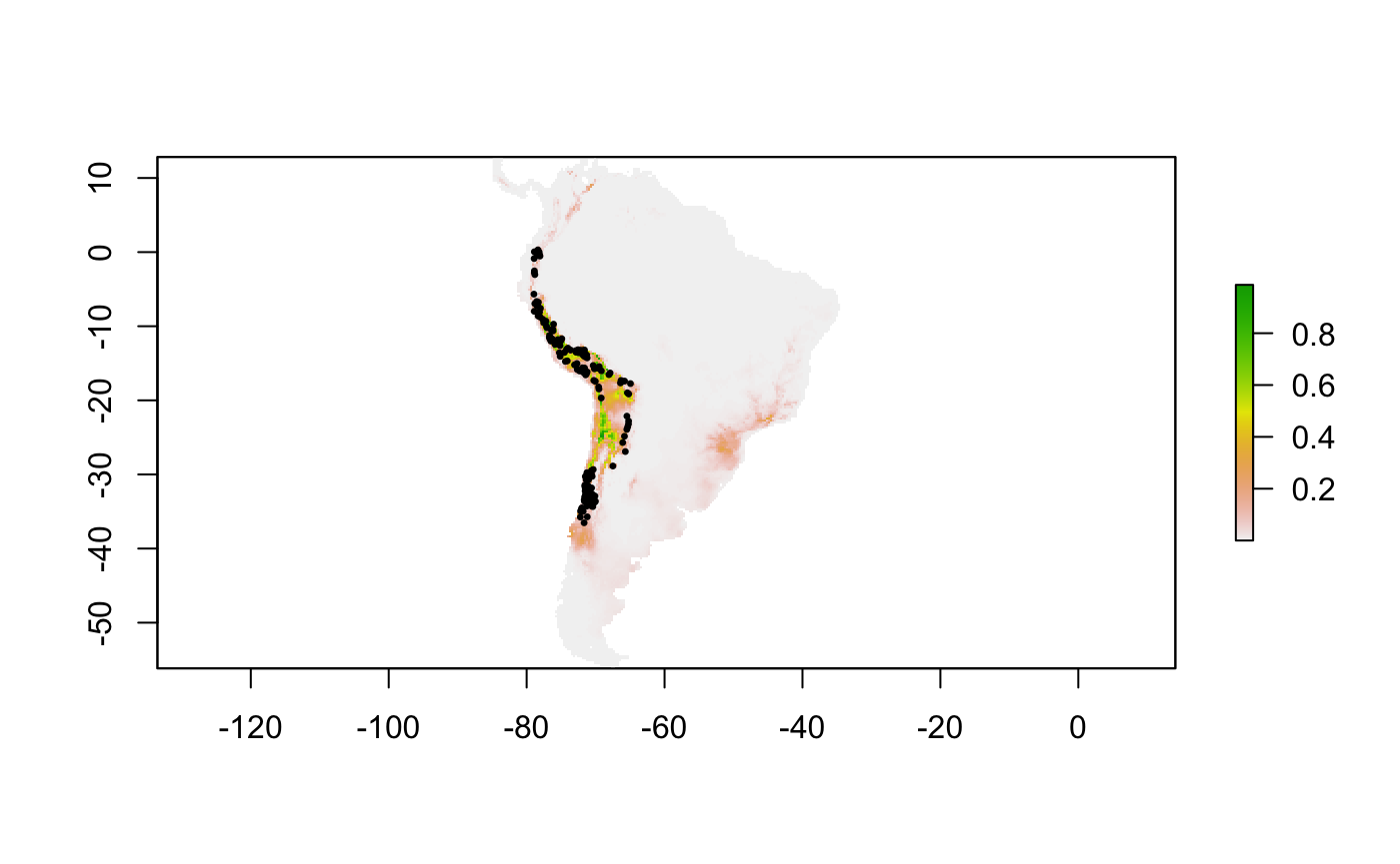
With the following lines of code, I am going to display the model in the first row of the table
# Best ellipsoid model for "omr_criteria"
bestvarcomb <- stringr::str_split(e_selct$fitted_vars,",")[[1]]

# Ellipsoid model (environmental space)
best_mod <- ntbox::cov_center(pg_etrain[,bestvarcomb],
                              mve = T,
                              level = 0.99,
                              vars = 1:length(bestvarcomb))


# Projection model in geographic space

mProj <- ntbox::ellipsoidfit(wc[[bestvarcomb]],
                             centroid = best_mod$centroid,
                             covar = best_mod$covariance,
                             level = 0.99,size = 3)
raster::plot(mProj$suitRaster)
points(pg[,c("longitude","latitude")],pch=20,cex=0.5)
References
Peterson, A. Townsend, Monica Papes, and Jorge Soberon. 2008. “Rethinking receiver operating characteristic analysis applications in ecological niche modeling.” Ecol. Modell. 213 (1): 63–72.
Van Aelst, Stefan, and Peter Rousseeuw. 2009. “Minimum volume ellipsoid.” Wiley Interdiscip. Rev. Comput. Stat. 1 (1): 71–82. https://doi.org/10.1002/wics.19.