predicts species' distribution under suitability changes
Usage
# S4 method for class 'bam'
predict(
  object,
  niche_layers,
  nbgs_vec = NULL,
  nsteps_vec,
  stochastic_dispersal = FALSE,
  disp_prop2_suitability = TRUE,
  disper_prop = 0.5,
  animate = FALSE,
  period_names = NULL,
  fmt = "GIF",
  filename,
  bg_color = "#F6F2E5",
  suit_color = "#0076BE",
  occupied_color = "#03C33F",
  png_keyword = "sdm_sim",
  ani.width = 1200,
  ani.height = 1200,
  ani.res = 300
)
Arguments
- object
a of class bam.
- niche_layers
A raster or RasterStack with the niche models for each time period
- nbgs_vec
A vector with the number of neighbors for the adjacency matrices
- nsteps_vec
Number of simulation steps for each time period.
- stochastic_dispersal
Logical. If dispersal depends on a probability of visiting neighbor cells (Moore neighborhood).
- disp_prop2_suitability
Logical. If probability of dispersal is proportional to the suitability of reachable cells. The proportional value must be declared in the parameter `disper_prop`.
- disper_prop
Probability of dispersal to reachable cells.
- animate
Logical. If TRUE a dispersal animation on climate change scenarios will be created
- period_names
Character vector with the names of periods that will be animated. Default NULL.
- fmt
Animation format. Possible values are GIF and HTML
- filename
File name.
- bg_color
Color for unsuitable pixels. Default "#F6F2E5".
- suit_color
Color for suitable pixels. Default "#0076BE".
- occupied_color
Color for occupied pixels. Default "#03C33F".
- png_keyword
A keyword name for the png images generated by the function
- ani.width
Animation width unit in px
- ani.height
Animation height unit in px
- ani.res
Animation resolution unit in px
Value
A RasterStack of predictions of dispersal dynamics as a function of environmental change scenarios.
Examples
# rm(list = ls())
# Read raster model for Lepus californicus
model_path <- system.file("extdata/Lepus_californicus_cont.tif",
package = "bamm")
model <- raster::raster(model_path)
# Convert model to sparse
sparse_mod <- bamm::model2sparse(model = model,threshold=0.1)
# Compute adjacency matrix
adj_mod <- bamm::adj_mat(sparse_mod,ngbs=1)
# Initial points to start dispersal process
occs_lep_cal <- data.frame(longitude = c(-115.10417,
-104.90417),
latitude = c(29.61846,
29.81846))
# Convert to sparse the initial points
occs_sparse <- bamm::occs2sparse(modelsparse = sparse_mod,
occs = occs_lep_cal)
# Run the bam (sdm) simultation for 100 time steps
smd_lep_cal <- bamm::sdm_sim(set_A = sparse_mod,
set_M = adj_mod,
initial_points = occs_sparse,
nsteps = 10)
#> Simulation progress:
#> [ ]
[
[====> ] 9%
[=========> ] 18%
[=============> ] 27%
[==================> ] 36%
[======================> ] 45%
[===========================> ] 54%
[===============================> ] 63%
[====================================> ] 72%
[========================================> ] 81%
[=============================================> ] 90%
[==================================================] 100%
#----------------------------------------------------------------------------
# Predict species' distribution under suitability change
# scenarios (could be climate chage scenarios).
#----------------------------------------------------------------------------
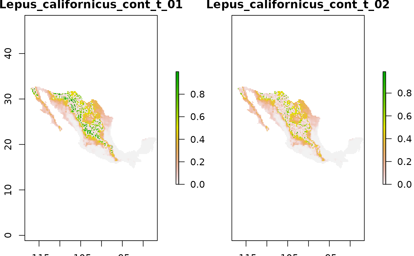
# Read suitability layers (two suitability change scenarios)
layers_path <- system.file("extdata/suit_change",
package = "bamm")
niche_mods_stack <- raster::stack(list.files(layers_path,
pattern = ".tif$",
full.names = TRUE))
raster::plot(niche_mods_stack)
 # Predict
new_preds <- predict(object = smd_lep_cal,
niche_layers = niche_mods_stack,
nsteps_vec = c(50,100))
#> Simulation progress:
#> [ ]
[
[> ] 1%
[=> ] 3%
[==> ] 5%
[===> ] 7%
[====> ] 9%
[=====> ] 11%
[======> ] 13%
[=======> ] 15%
[========> ] 17%
[=========> ] 19%
[==========> ] 21%
[===========> ] 23%
[============> ] 25%
[=============> ] 27%
[==============> ] 29%
[===============> ] 31%
[================> ] 33%
[=================> ] 35%
[==================> ] 37%
[===================> ] 39%
[====================> ] 41%
[=====================> ] 43%
[======================> ] 45%
[=======================> ] 47%
[========================> ] 49%
[=========================> ] 50%
[==========================> ] 52%
[===========================> ] 54%
[============================> ] 56%
[=============================> ] 58%
[==============================> ] 60%
[===============================> ] 62%
[================================> ] 64%
[=================================> ] 66%
[==================================> ] 68%
[===================================> ] 70%
[====================================> ] 72%
[=====================================> ] 74%
[======================================> ] 76%
[=======================================> ] 78%
[========================================> ] 80%
[=========================================> ] 82%
[==========================================> ] 84%
[===========================================> ] 86%
[============================================> ] 88%
[=============================================> ] 90%
[==============================================> ] 92%
[===============================================> ] 94%
[================================================> ] 96%
[=================================================>] 98%
[==================================================] 100%
#> Simulation progress:
#> [ ]
[
[> ] 1%
[=> ] 3%
[==> ] 5%
[===> ] 7%
[====> ] 9%
[=====> ] 11%
[======> ] 13%
[=======> ] 15%
[========> ] 17%
[=========> ] 19%
[==========> ] 21%
[===========> ] 23%
[============> ] 25%
[=============> ] 27%
[==============> ] 29%
[===============> ] 31%
[================> ] 33%
[=================> ] 35%
[==================> ] 37%
[===================> ] 39%
[====================> ] 41%
[=====================> ] 43%
[======================> ] 45%
[=======================> ] 47%
[========================> ] 49%
[=========================> ] 51%
[==========================> ] 53%
[===========================> ] 55%
[============================> ] 57%
[=============================> ] 59%
[==============================> ] 61%
[===============================> ] 63%
[================================> ] 65%
[=================================> ] 67%
[==================================> ] 69%
[===================================> ] 71%
[====================================> ] 73%
[=====================================> ] 75%
[======================================> ] 77%
[=======================================> ] 79%
[========================================> ] 81%
[=========================================> ] 83%
[==========================================> ] 85%
[===========================================> ] 87%
[============================================> ] 89%
[=============================================> ] 91%
[==============================================> ] 93%
[===============================================> ] 95%
[================================================> ] 97%
[=================================================>] 99%
[==================================================] 100%
# Generate the dispersal animation for time period 1 and 2
# \donttest{
if(requireNamespace("animation")){
ani_prd <- tempfile(pattern = "prediction_",fileext = ".gif")
#new_preds <- predict(object = smd_lep_cal,
# niche_layers = niche_mods_stack,
# nsteps_vec = c(10,10),
# animate=TRUE,
# filename=ani_prd,
# fmt="GIF")
}
# }
# Predict
new_preds <- predict(object = smd_lep_cal,
niche_layers = niche_mods_stack,
nsteps_vec = c(50,100))
#> Simulation progress:
#> [ ]
[
[> ] 1%
[=> ] 3%
[==> ] 5%
[===> ] 7%
[====> ] 9%
[=====> ] 11%
[======> ] 13%
[=======> ] 15%
[========> ] 17%
[=========> ] 19%
[==========> ] 21%
[===========> ] 23%
[============> ] 25%
[=============> ] 27%
[==============> ] 29%
[===============> ] 31%
[================> ] 33%
[=================> ] 35%
[==================> ] 37%
[===================> ] 39%
[====================> ] 41%
[=====================> ] 43%
[======================> ] 45%
[=======================> ] 47%
[========================> ] 49%
[=========================> ] 50%
[==========================> ] 52%
[===========================> ] 54%
[============================> ] 56%
[=============================> ] 58%
[==============================> ] 60%
[===============================> ] 62%
[================================> ] 64%
[=================================> ] 66%
[==================================> ] 68%
[===================================> ] 70%
[====================================> ] 72%
[=====================================> ] 74%
[======================================> ] 76%
[=======================================> ] 78%
[========================================> ] 80%
[=========================================> ] 82%
[==========================================> ] 84%
[===========================================> ] 86%
[============================================> ] 88%
[=============================================> ] 90%
[==============================================> ] 92%
[===============================================> ] 94%
[================================================> ] 96%
[=================================================>] 98%
[==================================================] 100%
#> Simulation progress:
#> [ ]
[
[> ] 1%
[=> ] 3%
[==> ] 5%
[===> ] 7%
[====> ] 9%
[=====> ] 11%
[======> ] 13%
[=======> ] 15%
[========> ] 17%
[=========> ] 19%
[==========> ] 21%
[===========> ] 23%
[============> ] 25%
[=============> ] 27%
[==============> ] 29%
[===============> ] 31%
[================> ] 33%
[=================> ] 35%
[==================> ] 37%
[===================> ] 39%
[====================> ] 41%
[=====================> ] 43%
[======================> ] 45%
[=======================> ] 47%
[========================> ] 49%
[=========================> ] 51%
[==========================> ] 53%
[===========================> ] 55%
[============================> ] 57%
[=============================> ] 59%
[==============================> ] 61%
[===============================> ] 63%
[================================> ] 65%
[=================================> ] 67%
[==================================> ] 69%
[===================================> ] 71%
[====================================> ] 73%
[=====================================> ] 75%
[======================================> ] 77%
[=======================================> ] 79%
[========================================> ] 81%
[=========================================> ] 83%
[==========================================> ] 85%
[===========================================> ] 87%
[============================================> ] 89%
[=============================================> ] 91%
[==============================================> ] 93%
[===============================================> ] 95%
[================================================> ] 97%
[=================================================>] 99%
[==================================================] 100%
# Generate the dispersal animation for time period 1 and 2
# \donttest{
if(requireNamespace("animation")){
ani_prd <- tempfile(pattern = "prediction_",fileext = ".gif")
#new_preds <- predict(object = smd_lep_cal,
# niche_layers = niche_mods_stack,
# nsteps_vec = c(10,10),
# animate=TRUE,
# filename=ani_prd,
# fmt="GIF")
}
# }