sdm_sim: Simulate single species dispersal dynamics using the BAM framework.
Source:R/sdm_sim.R
sdm_sim.Rdsdm_sim: Simulate single species dispersal dynamics using the BAM framework.
Usage
sdm_sim(
  set_A,
  set_M,
  sp_interaction_model = NULL,
  initial_points,
  nsteps,
  stochastic_dispersal = TRUE,
  disp_prop2_suitability = TRUE,
  disper_prop = 0.5,
  progress_bar = TRUE,
  rcpp = TRUE
)
Arguments
- set_A
A setA object returned by the function
model2sparse- set_M
A setM object containing the adjacency matrix of the study area. See
adj_mat- sp_interaction_model
A RasterLayer representing a suitability model of a species positive interaction. See details
- initial_points
A sparse vector returned by the function
occs2sparse- nsteps
Number of steps to run the simulation
- stochastic_dispersal
Logical. If dispersal depends on a probability of visiting neighbor cells (Moore neighborhood).
- disp_prop2_suitability
Logical. If probability of dispersal is proportional to the suitability of reachable cells. The proportional value must be declared in the parameter `disper_prop`.
- disper_prop
Probability of dispersal to reachable cells.
- progress_bar
Show progress bar
- rcpp
Logical. Use native C++ code to run the model.
Value
An object of class bam with simulation results.
The simulation are stored in the sdm_sim slot (a list of sparse matrices).
Details
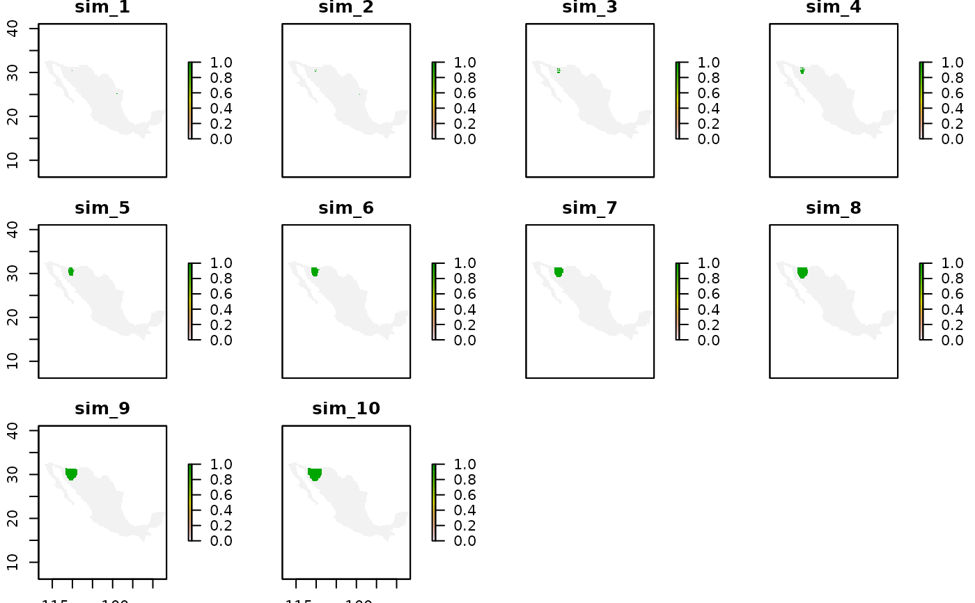
The model is cellular automata where the occupied area of a species at time \(t+1\) is estimated by the multiplication of two binary matrices: one matrix represents movements (M), another abiotic -niche- tolerances (A) (Soberon and Osorio-Olvera, 2022). $$\mathbf{G}_j(t+1) =\mathbf{A}_j(t)\mathbf{M}_j \mathbf{G}_j(t)$$ The equation describes a very simple process: To find the occupied patches in \(t+1\) start with those occupied at time \(t\) denoted by \(\mathbf{G}_j(t)\), allow the individuals to disperse among adjacent patches, as defined by \(\mathbf{M}_j\), then remove individuals from patches that are unsuitable, as defined by \(\mathbf{A}_j(t)\).
The stochastic model uses a suitability values to model dispersal probabilities. These suitability values can be either obtained from the continues model stored in the set_A object or from the sp_interaction_model (RasterLayer). If the parameter rcpp is set to TRUE the model will be run using native C++ code through Rcpp and RcppArmadillo packages.
References
Soberón J, Osorio-Olvera L (2023). “A dynamic theory of the area of distribution.” Journal of Biogeography6, 50, 1037-1048. doi:10.1111/jbi.14587 , https://onlinelibrary.wiley.com/doi/abs/10.1111/jbi.14587. .
Examples
# \donttest{
model_path <- system.file("extdata/Lepus_californicus_cont.tif",
package = "bamm")
model <- raster::raster(model_path)
sparse_mod <- bamm::model2sparse(model,threshold=0.05)
adj_mod <- bamm::adj_mat(sparse_mod,ngbs=1)
occs_lep_cal <- data.frame(longitude = c(-110.08880,
-98.89638),
latitude = c(30.43455,
25.19919))
occs_sparse <- bamm::occs2sparse(modelsparse = sparse_mod,
occs = occs_lep_cal)
sdm_lep_cal <- bamm::sdm_sim(set_A = sparse_mod,
set_M = adj_mod,
initial_points = occs_sparse,
nsteps = 100,
stochastic_dispersal = TRUE,
disp_prop2_suitability=FALSE,
disper_prop=0.5,
progress_bar=TRUE)
#> Simulation progress:
#> [ ]
[
[> ] 1%
[=> ] 3%
[==> ] 5%
[===> ] 7%
[====> ] 9%
[=====> ] 11%
[======> ] 13%
[=======> ] 15%
[========> ] 17%
[=========> ] 19%
[==========> ] 21%
[===========> ] 23%
[============> ] 25%
[=============> ] 27%
[==============> ] 29%
[===============> ] 31%
[================> ] 33%
[=================> ] 35%
[==================> ] 37%
[===================> ] 39%
[====================> ] 41%
[=====================> ] 43%
[======================> ] 45%
[=======================> ] 47%
[========================> ] 49%
[=========================> ] 51%
[==========================> ] 53%
[===========================> ] 55%
[============================> ] 57%
[=============================> ] 59%
[==============================> ] 61%
[===============================> ] 63%
[================================> ] 65%
[=================================> ] 67%
[==================================> ] 69%
[===================================> ] 71%
[====================================> ] 73%
[=====================================> ] 75%
[======================================> ] 77%
[=======================================> ] 79%
[========================================> ] 81%
[=========================================> ] 83%
[==========================================> ] 85%
[===========================================> ] 87%
[============================================> ] 89%
[=============================================> ] 91%
[==============================================> ] 93%
[===============================================> ] 95%
[================================================> ] 97%
[=================================================>] 99%
[==================================================] 100%
sim_res <- bamm::sim2Raster(sdm_lep_cal)
#>
|
| | 0%
|
|= | 1%
|
|= | 2%
|
|== | 3%
|
|=== | 4%
|
|==== | 5%
|
|==== | 6%
|
|===== | 7%
|
|====== | 8%
|
|====== | 9%
|
|======= | 10%
|
|======== | 11%
|
|======== | 12%
|
|========= | 13%
|
|========== | 14%
|
|========== | 15%
|
|=========== | 16%
|
|============ | 17%
|
|============= | 18%
|
|============= | 19%
|
|============== | 20%
|
|=============== | 21%
|
|=============== | 22%
|
|================ | 23%
|
|================= | 24%
|
|================== | 25%
|
|================== | 26%
|
|=================== | 27%
|
|==================== | 28%
|
|==================== | 29%
|
|===================== | 30%
|
|====================== | 31%
|
|====================== | 32%
|
|======================= | 33%
|
|======================== | 34%
|
|======================== | 35%
|
|========================= | 36%
|
|========================== | 37%
|
|=========================== | 38%
|
|=========================== | 39%
|
|============================ | 40%
|
|============================= | 41%
|
|============================= | 42%
|
|============================== | 43%
|
|=============================== | 44%
|
|================================ | 45%
|
|================================ | 46%
|
|================================= | 47%
|
|================================== | 48%
|
|================================== | 49%
|
|=================================== | 50%
|
|==================================== | 51%
|
|==================================== | 52%
|
|===================================== | 53%
|
|====================================== | 54%
|
|====================================== | 55%
|
|======================================= | 56%
|
|======================================== | 57%
|
|========================================= | 58%
|
|========================================= | 59%
|
|========================================== | 60%
|
|=========================================== | 61%
|
|=========================================== | 62%
|
|============================================ | 63%
|
|============================================= | 64%
|
|============================================== | 65%
|
|============================================== | 66%
|
|=============================================== | 67%
|
|================================================ | 68%
|
|================================================ | 69%
|
|================================================= | 70%
|
|================================================== | 71%
|
|================================================== | 72%
|
|=================================================== | 73%
|
|==================================================== | 74%
|
|==================================================== | 75%
|
|===================================================== | 76%
|
|====================================================== | 77%
|
|======================================================= | 78%
|
|======================================================= | 79%
|
|======================================================== | 80%
|
|========================================================= | 81%
|
|========================================================= | 82%
|
|========================================================== | 83%
|
|=========================================================== | 84%
|
|============================================================ | 85%
|
|============================================================ | 86%
|
|============================================================= | 87%
|
|============================================================== | 88%
|
|============================================================== | 89%
|
|=============================================================== | 90%
|
|================================================================ | 91%
|
|================================================================ | 92%
|
|================================================================= | 93%
|
|================================================================== | 94%
|
|================================================================== | 95%
|
|=================================================================== | 96%
|
|==================================================================== | 97%
|
|===================================================================== | 98%
|
|===================================================================== | 99%
|
|======================================================================| 100%
raster::plot(sim_res)
 # }
# }